train_data <- read.csv("data/raw/challenge_training.data.prepared_data.csv")
test_data <- read.csv("data/raw/challenge_validation.data.prepared_data.csv")10 Model evaluation and selection
10.1 Model selection with information criteria
To demonstrate model selection we will use a dataset from a yield prediction challenge in 2015. The data comes from maize farms in Ethiopia. The data is split into two subsets, one for training models (i.e., estimating their coefficients) and one for testing the predicitons of the models:
Both datasets have the columns, they just represents different locations where yields were collected. There are a large number of columns in the dataset but, for simplicity, we are going to reduce the dimensions of the problem for the purpose of this practical. Let’s remove all the columns that include the word "rain" in their name. We first identify the columns that include the word "rain" with the function grep() and then remove them from the dataset:
rain_columns <- grep("rain", colnames(train_data))
train_data <- train_data[, -rain_columns]
test_data <- test_data[, -rain_columns]
To further simplify the exercise, we are going to select some variables based on prior research (that we know will be useful in any model) plus some additional random variables to have enough predictors to make the exercise interesting. The variables to be used based on prior research are as follows:
vars <- c("EVI","precip.PC9", "precip.PC8","precip.PC5", "total.precip","sndppt",
"precip.PC1","precip.PC17","precip.PC10","LSTD", "LSTN","clyppt", "drougth.days","sltppt",
"cecsol","sndppt", "drought", "taxnwrb_250m", "RED", "NIR", "EVI16")
The additional random variables are taken from the columns that have not been selected yet. We can determine which columns have not been selected by taking the set difference between the columns in the dataset and the columns that we have selected (we also include the variable we want to predict, "maizeyield"):
possible_vars <- setdiff(colnames(train_data), c(vars, "maizeyield"))Then we sample 5 of those variables:
set.seed(123)
random_vars <- sample(possible_vars, 5, replace = FALSE)
The final set of variables to be used for the exercise is the combination of the two sets:
vars <- c(vars, random_vars)A further step that is always good to do is to check for highly correlated variables. We can do this by calculating the correlation matrix of the predictors and then selecting the variables that have a correlation coefficient higher than 0.9:
cor.mat <- cor(train_data[,vars])
library(caret) # for findCorrelation()
Warning: package 'caret' was built under R version 4.4.1Loading required package: ggplot2Loading required package: latticehighly_correlated <- findCorrelation(cor.mat, cutoff = 0.9) # highly correlated variables
vars <- setdiff(vars, row.names(cor.mat)[highly_correlated])We could already fit a linear model that includes all these predictors. Instead of typing a very long formula, we can create a formula as text and then evaluate it:
formula <- as.formula(paste("maizeyield ~", paste(vars, collapse = " + ")))
formula
maizeyield ~ EVI + precip.PC9 + precip.PC8 + precip.PC5 + precip.PC1 +
precip.PC17 + precip.PC10 + LSTD + LSTN + clyppt + drougth.days +
sltppt + cecsol + drought + taxnwrb_250m + NIR + MIR + sub_mg +
sub_k + altitude + precip.PC11We could use this formula in a linear model already:
lm_model <- lm(formula, data = train_data)
summary(lm_model)
Call:
lm(formula = formula, data = train_data)
Residuals:
Min 1Q Median 3Q Max
-3063.4 -1018.6 -71.6 942.6 5752.7
Coefficients:
Estimate Std. Error t value Pr(>|t|)
(Intercept) 717.1371 10444.7352 0.069 0.9454
EVI 2.6095 1.6995 1.535 0.1276
precip.PC9 -41.5509 63.6775 -0.653 0.5155
precip.PC8 -25.1229 31.6826 -0.793 0.4296
precip.PC5 -73.2075 50.2255 -1.458 0.1479
precip.PC1 -8.7730 12.0302 -0.729 0.4674
precip.PC17 -103.6781 77.5636 -1.337 0.1842
precip.PC10 39.9497 63.9966 0.624 0.5338
LSTD -140.5604 163.7996 -0.858 0.3927
LSTN 170.0015 305.1148 0.557 0.5786
clyppt -13.1818 89.5905 -0.147 0.8833
drougth.days -244.2014 296.7224 -0.823 0.4123
sltppt -30.9773 142.4446 -0.217 0.8283
cecsol 34.7902 38.5396 0.903 0.3687
drought 1641.5384 987.7678 1.662 0.0995 .
taxnwrb_250m 10.7345 6.4596 1.662 0.0995 .
NIR -4.0099 3.1886 -1.258 0.2113
MIR 3.6838 2.2835 1.613 0.1096
sub_mg -0.8441 1.5956 -0.529 0.5979
sub_k -1.4258 1.8344 -0.777 0.4387
altitude 0.9925 1.5832 0.627 0.5321
precip.PC11 -7.7927 83.3678 -0.093 0.9257
---
Signif. codes: 0 '***' 0.001 '**' 0.01 '*' 0.05 '.' 0.1 ' ' 1
Residual standard error: 1562 on 107 degrees of freedom
Multiple R-squared: 0.3708, Adjusted R-squared: 0.2473
F-statistic: 3.003 on 21 and 107 DF, p-value: 0.0001079An R2 of 0.37 is a bit underwhelming but it is a good starting point. We are now going to extend this linear model by including a spatial correlation structure. That is, we want to add the effect of longitude and latitude to the model as predictors, but we also want to account for the fact that the residuals of the model are likely to be spatially correlated. Note that adding the spatial coordinates to a model is useful when the goal is to perform spatial interpolation (i.e., predict the yield at locations where we do not have data) or for predictions in the same region for future years.
We know we can add this correlation structure using lme() from the nlme package. However, this package requires at least one random effect in order to work. To trick R, we can create a dummy variable (that has the same value for all observations) and use it as the random effect. This will keep lme() happy and allow us to fit the model:
train_data$dummy <- 1
test_data$dummy <- 1Now we can fit a mixed effect model with the spatial correlation structure (corMatern) from the package spaMM:
library(nlme)
library(spaMM)Warning: package 'spaMM' was built under R version 4.4.1Registered S3 methods overwritten by 'registry':
method from
print.registry_field proxy
print.registry_entry proxyspaMM (Rousset & Ferdy, 2014, version 4.5.0) is loaded.
Type 'help(spaMM)' for a short introduction,
'news(package='spaMM')' for news,
and 'citation('spaMM')' for proper citation.
Further infos, slides, etc. at https://gitlab.mbb.univ-montp2.fr/francois/spamm-ref.full_model <- lme(fixed = formula, data = train_data, random = ~1 | dummy,
correlation = corMatern(form = ~longitude + latitude | dummy),
method = "ML")We can already compare the two models using the AIC:
c(AIC(lm_model), AIC(full_model))[1] 2285.250 2288.788Adding the correlation structure has not improved the model. However, we still have a lot of predictors in the model. We can use the stepAIC() function to perform a stepwise selection of the predictors using AIC as the criterion. This will start with the full model and remove predictors one by one until the AIC is minimized (so we are doing backward selection). This will take some time to run:
library(MASS)
step_model <- stepAIC(full_model, direction = "backward", k =2)Start: AIC=2288.79
maizeyield ~ EVI + precip.PC9 + precip.PC8 + precip.PC5 + precip.PC1 +
    precip.PC17 + precip.PC10 + LSTD + LSTN + clyppt + drougth.days +
    sltppt + cecsol + drought + taxnwrb_250m + NIR + MIR + sub_mg +
    sub_k + altitude + precip.PC11
Df AIC
- precip.PC11 1 2286.8
- clyppt 1 2286.8
- sltppt 1 2287.0
- altitude 1 2287.0
- precip.PC9 1 2287.1
- sub_k 1 2287.1
- LSTN 1 2287.2
- precip.PC10 1 2287.3
- drougth.days 1 2287.3
- precip.PC1 1 2287.3
- sub_mg 1 2287.3
- precip.PC8 1 2287.3
- LSTD 1 2287.7
- cecsol 1 2287.7
- precip.PC5 1 2288.1
- NIR 1 2288.1
- precip.PC17 1 2288.2
<none> 2288.8
- drought 1 2288.9
- EVI 1 2289.1
- taxnwrb_250m 1 2289.4
- MIR 1 2289.5
Step: AIC=2286.79
maizeyield ~ EVI + precip.PC9 + precip.PC8 + precip.PC5 + precip.PC1 +
precip.PC17 + precip.PC10 + LSTD + LSTN + clyppt + drougth.days +
sltppt + cecsol + drought + taxnwrb_250m + NIR + MIR + sub_mg +
sub_k + altitude
Df AIC
- clyppt 1 2284.8
- sltppt 1 2285.0
- altitude 1 2285.1
- precip.PC9 1 2285.1
- sub_k 1 2285.1
- precip.PC1 1 2285.3
- LSTN 1 2285.3
- sub_mg 1 2285.3
- precip.PC8 1 2285.5
- drougth.days 1 2285.5
- precip.PC10 1 2285.6
- cecsol 1 2285.7
- LSTD 1 2285.8
- NIR 1 2286.1
- precip.PC17 1 2286.3
<none> 2286.8
- EVI 1 2287.2
- drought 1 2287.2
- taxnwrb_250m 1 2287.4
- MIR 1 2287.5
- precip.PC5 1 2289.3
Step: AIC=2284.81
maizeyield ~ EVI + precip.PC9 + precip.PC8 + precip.PC5 + precip.PC1 +
precip.PC17 + precip.PC10 + LSTD + LSTN + drougth.days +
sltppt + cecsol + drought + taxnwrb_250m + NIR + MIR + sub_mg +
sub_k + altitude
Df AIC
- sltppt 1 2283.0
- altitude 1 2283.1
- precip.PC9 1 2283.1
- sub_k 1 2283.1
- precip.PC1 1 2283.3
- sub_mg 1 2283.3
- LSTN 1 2283.4
- precip.PC8 1 2283.5
- drougth.days 1 2283.6
- cecsol 1 2283.8
- precip.PC10 1 2283.8
- LSTD 1 2283.9
- NIR 1 2284.1
- precip.PC17 1 2284.3
<none> 2284.8
- EVI 1 2285.2
- drought 1 2285.2
- taxnwrb_250m 1 2285.5
- MIR 1 2285.7
- precip.PC5 1 2287.4
Step: AIC=2282.99
maizeyield ~ EVI + precip.PC9 + precip.PC8 + precip.PC5 + precip.PC1 +
precip.PC17 + precip.PC10 + LSTD + LSTN + drougth.days +
cecsol + drought + taxnwrb_250m + NIR + MIR + sub_mg + sub_k +
altitude
Df AIC
- altitude 1 2281.2
- precip.PC9 1 2281.3
- sub_k 1 2281.4
- sub_mg 1 2281.4
- LSTN 1 2281.6
- precip.PC1 1 2281.7
- precip.PC8 1 2281.7
- drougth.days 1 2281.7
- cecsol 1 2281.8
- precip.PC10 1 2281.9
- LSTD 1 2282.2
- precip.PC17 1 2282.4
- NIR 1 2282.4
<none> 2283.0
- EVI 1 2283.3
- drought 1 2283.5
- MIR 1 2283.7
- taxnwrb_250m 1 2284.0
- precip.PC5 1 2285.6
Step: AIC=2281.25
maizeyield ~ EVI + precip.PC9 + precip.PC8 + precip.PC5 + precip.PC1 +
precip.PC17 + precip.PC10 + LSTD + LSTN + drougth.days +
cecsol + drought + taxnwrb_250m + NIR + MIR + sub_mg + sub_k
Df AIC
- precip.PC9 1 2279.5
- LSTN 1 2279.6
- sub_k 1 2279.6
- sub_mg 1 2279.7
- drougth.days 1 2279.8
- precip.PC1 1 2279.8
- precip.PC8 1 2279.8
- precip.PC10 1 2280.1
- cecsol 1 2280.3
- NIR 1 2280.4
- precip.PC17 1 2280.6
- LSTD 1 2280.9
<none> 2281.2
- EVI 1 2281.3
- drought 1 2281.7
- MIR 1 2281.7
- taxnwrb_250m 1 2282.0
- precip.PC5 1 2283.7
Step: AIC=2279.54
maizeyield ~ EVI + precip.PC8 + precip.PC5 + precip.PC1 + precip.PC17 +
precip.PC10 + LSTD + LSTN + drougth.days + cecsol + drought +
taxnwrb_250m + NIR + MIR + sub_mg + sub_k
Df AIC
- LSTN 1 2277.7
- sub_k 1 2277.8
- drougth.days 1 2277.9
- sub_mg 1 2278.0
- cecsol 1 2278.3
- precip.PC1 1 2278.3
- precip.PC10 1 2278.4
- NIR 1 2278.5
- precip.PC8 1 2278.6
- precip.PC17 1 2278.8
- LSTD 1 2278.9
- EVI 1 2279.4
<none> 2279.5
- MIR 1 2279.7
- drought 1 2279.7
- taxnwrb_250m 1 2280.1
- precip.PC5 1 2281.7
Step: AIC=2277.72
maizeyield ~ EVI + precip.PC8 + precip.PC5 + precip.PC1 + precip.PC17 +
precip.PC10 + LSTD + drougth.days + cecsol + drought + taxnwrb_250m +
NIR + MIR + sub_mg + sub_k
Df AIC
- sub_k 1 2276.0
- sub_mg 1 2276.2
- cecsol 1 2276.3
- drougth.days 1 2276.4
- precip.PC8 1 2276.6
- precip.PC10 1 2276.7
- NIR 1 2276.9
- LSTD 1 2277.0
- precip.PC17 1 2277.3
- precip.PC1 1 2277.4
<none> 2277.7
- EVI 1 2277.9
- MIR 1 2278.2
- drought 1 2278.2
- taxnwrb_250m 1 2278.3
- precip.PC5 1 2282.6
Step: AIC=2275.97
maizeyield ~ EVI + precip.PC8 + precip.PC5 + precip.PC1 + precip.PC17 +
precip.PC10 + LSTD + drougth.days + cecsol + drought + taxnwrb_250m +
NIR + MIR + sub_mg
Df AIC
- cecsol 1 2274.5
- drougth.days 1 2274.7
- sub_mg 1 2274.7
- precip.PC8 1 2274.9
- NIR 1 2275.1
- LSTD 1 2275.2
- precip.PC10 1 2275.2
- precip.PC17 1 2275.6
- precip.PC1 1 2275.7
<none> 2276.0
- EVI 1 2276.0
- MIR 1 2276.3
- drought 1 2276.3
- taxnwrb_250m 1 2276.7
- precip.PC5 1 2280.7
Step: AIC=2274.5
maizeyield ~ EVI + precip.PC8 + precip.PC5 + precip.PC1 + precip.PC17 +
precip.PC10 + LSTD + drougth.days + drought + taxnwrb_250m +
NIR + MIR + sub_mg
Df AIC
- drougth.days 1 2273.1
- precip.PC8 1 2273.3
- sub_mg 1 2273.3
- LSTD 1 2273.5
- NIR 1 2273.5
- precip.PC10 1 2273.6
- precip.PC17 1 2273.7
- EVI 1 2274.3
- precip.PC1 1 2274.4
<none> 2274.5
- drought 1 2274.7
- taxnwrb_250m 1 2274.9
- MIR 1 2274.9
- precip.PC5 1 2278.7
Step: AIC=2273.06
maizeyield ~ EVI + precip.PC8 + precip.PC5 + precip.PC1 + precip.PC17 +
precip.PC10 + LSTD + drought + taxnwrb_250m + NIR + MIR +
sub_mg
Df AIC
- precip.PC8 1 2271.4
- precip.PC17 1 2271.8
- sub_mg 1 2272.1
- precip.PC10 1 2272.2
- LSTD 1 2272.2
- NIR 1 2272.8
<none> 2273.1
- taxnwrb_250m 1 2273.1
- MIR 1 2273.6
- drought 1 2273.6
- precip.PC1 1 2273.8
- EVI 1 2273.8
- precip.PC5 1 2276.9
Step: AIC=2271.36
maizeyield ~ EVI + precip.PC5 + precip.PC1 + precip.PC17 + precip.PC10 +
LSTD + drought + taxnwrb_250m + NIR + MIR + sub_mg
Df AIC
- precip.PC17 1 2270.2
- precip.PC10 1 2270.3
- sub_mg 1 2270.7
- LSTD 1 2271.0
<none> 2271.4
- drought 1 2271.8
- taxnwrb_250m 1 2271.8
- NIR 1 2272.1
- MIR 1 2272.2
- EVI 1 2272.6
- precip.PC1 1 2273.2
- precip.PC5 1 2275.2
Step: AIC=2270.24
maizeyield ~ EVI + precip.PC5 + precip.PC1 + precip.PC10 + LSTD +
drought + taxnwrb_250m + NIR + MIR + sub_mg
Df AIC
- precip.PC10 1 2268.4
- sub_mg 1 2269.4
- LSTD 1 2269.6
<none> 2270.2
- taxnwrb_250m 1 2270.9
- NIR 1 2271.2
- MIR 1 2272.7
- EVI 1 2272.8
- drought 1 2272.8
- precip.PC5 1 2275.2
- precip.PC1 1 2277.2
Step: AIC=2268.44
maizeyield ~ EVI + precip.PC5 + precip.PC1 + LSTD + drought +
taxnwrb_250m + NIR + MIR + sub_mg
Df AIC
- sub_mg 1 2267.6
- LSTD 1 2268.2
<none> 2268.4
- taxnwrb_250m 1 2268.9
- NIR 1 2269.7
- MIR 1 2270.9
- EVI 1 2271.1
- drought 1 2271.3
- precip.PC5 1 2273.2
- precip.PC1 1 2275.9
Step: AIC=2267.57
maizeyield ~ EVI + precip.PC5 + precip.PC1 + LSTD + drought +
taxnwrb_250m + NIR + MIR
Df AIC
<none> 2267.6
- LSTD 1 2267.7
- taxnwrb_250m 1 2268.2
- NIR 1 2268.7
- MIR 1 2270.1
- EVI 1 2270.1
- drought 1 2270.2
- precip.PC5 1 2272.6
- precip.PC1 1 2277.2step_modelLinear mixed-effects model fit by maximum likelihood
Data: train_data
Log-likelihood: -1120.783
Fixed: maizeyield ~ EVI + precip.PC5 + precip.PC1 + LSTD + drought + taxnwrb_250m + NIR + MIR
(Intercept) EVI precip.PC5 precip.PC1 LSTD drought
2442.699605 2.504254 -54.419094 -24.515219 -136.640292 940.701870
taxnwrb_250m NIR MIR
8.429614 -4.109523 3.831153
Random effects:
Formula: ~1 | dummy
(Intercept) Residual
StdDev: 0.09071041 1476.319
Correlation Structure: corMatern
Formula: ~longitude + latitude | dummy
Parameter estimate(s):
range nu
0.01277368 0.10454763
Number of Observations: 129
Number of Groups: 1 We can see that the selected model is much smaller than the full model. We can now compare the AIC of the three models so far:
c(AIC(lm_model), AIC(full_model), AIC(step_model))[1] 2285.250 2288.788 2267.567An improvement of about 20 AIC units is quite a significant improvement. We can visualize the performance of the model by plotting observed versus predicted values. Let’s do that for the full model:
pred_full <- predict(full_model)
eval_full <- lm(train_data$maizeyield~pred_full)
summary(eval_full)
Call:
lm(formula = train_data$maizeyield ~ pred_full)

Residuals:
    Min      1Q  Median      3Q     Max
-2996.4 -1051.2  -135.0   994.6  5727.9

Coefficients:
            Estimate Std. Error t value Pr(>|t|)
(Intercept)  25.0253   445.4382   0.056    0.955
pred_full     0.9983     0.1160   8.603  2.5e-14 ***
---
Signif. codes:  0 '***' 0.001 '**' 0.01 '*' 0.05 '.' 0.1 ' ' 1

Residual standard error: 1437 on 127 degrees of freedom
Multiple R-squared:  0.3682,    Adjusted R-squared:  0.3632
F-statistic: 74 on 1 and 127 DF, p-value: 2.504e-14plot(train_data$maizeyield~pred_full, ylab = "Observed", xlab = "Predicted",
xlim = c(0, 13e3), ylim = c(0, 13e3))
abline(eval_full)
abline(a = 0, b = 1, col = "red")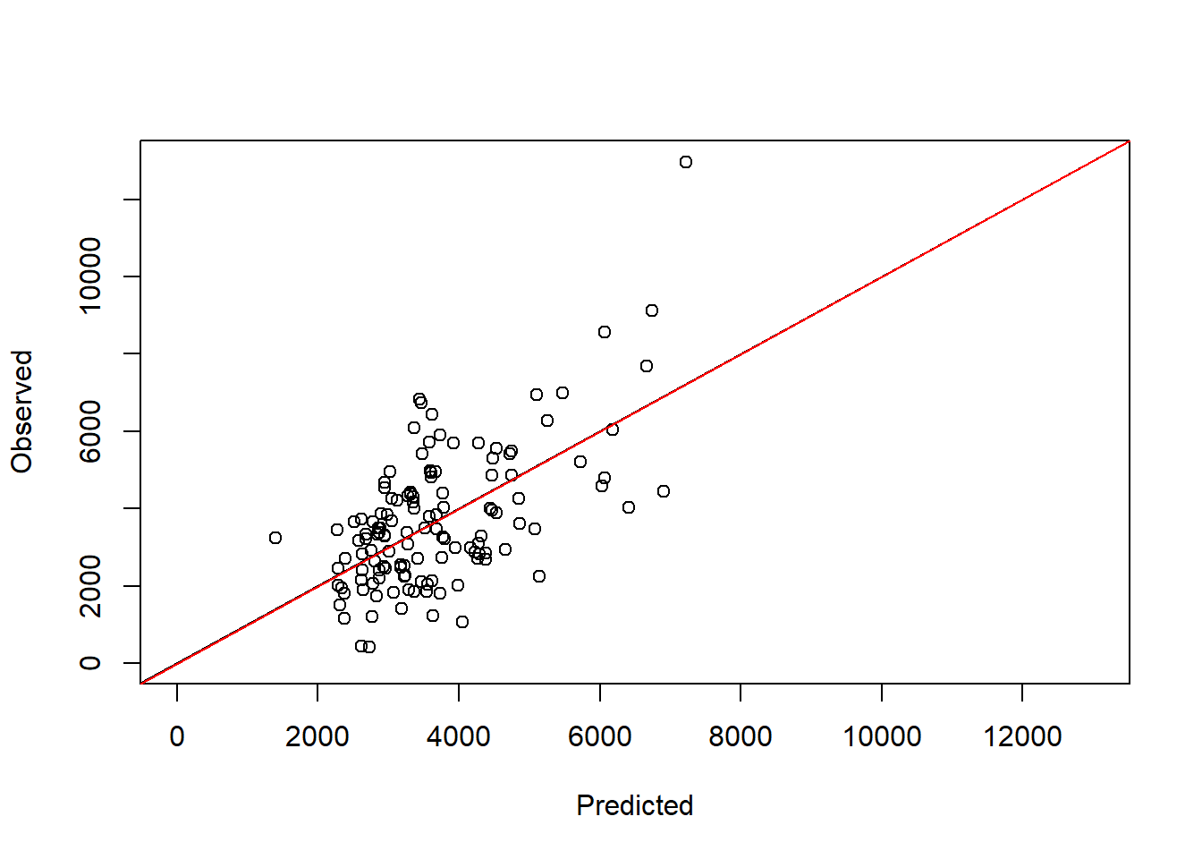
We can see that the slope is very close to 1 and the intercept is not different from 0 statistically speaking. Indeed, the regression line is very close to the 1:1 line. This implies that there are no significant biases in the fitted model (at least when compared to the training data). A more honest evaluation of the model would be to use the test data instead. This is easy to achieve by assigning the correct argument inside predict():
full_model$call$fixed <- formula # deal with obscure bug in predict, ask Alejandro
pred_full <- predict(full_model, newdata = test_data)
eval_full <- lm(test_data$maizeyield~pred_full)
summary(eval_full)
Call:
lm(formula = test_data$maizeyield ~ pred_full)

Residuals:
    Min      1Q  Median      3Q     Max
-3457.0  -917.0    97.9  1041.2  2590.8

Coefficients:
             Estimate Std. Error t value Pr(>|t|)
(Intercept) 2786.1337   384.4109   7.248 6.32e-10 ***
pred_full      0.5392     0.1459   3.696 0.000452 ***
---
Signif. codes:  0 '***' 0.001 '**' 0.01 '*' 0.05 '.' 0.1 ' ' 1

Residual standard error: 1364 on 65 degrees of freedom
Multiple R-squared:  0.1737,    Adjusted R-squared:  0.1609
F-statistic: 13.66 on 1 and 65 DF, p-value: 0.0004517plot(test_data$maizeyield~pred_full, ylab = "Observed", xlab = "Predicted",
xlim = c(0, 8e3), ylim = c(0, 8e3))
abline(eval_full)
abline(a = 0, b = 1, col = "red")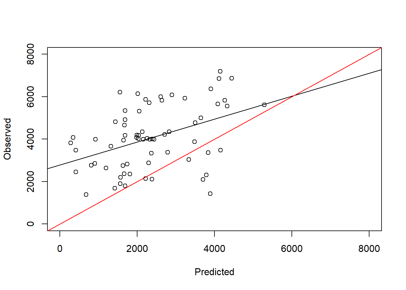
Indeed now we can see that the slope is no longer close to 1 and the intercept is larger than zero. This means that the model underestimates predicted yields in an independent dataset from the original one. The fact that the performance is much worse in the test dataset compared to the train dataset is a sign of overfitting. This is a common problem in machine learning and statistics. The model is too complex and captures noise in the training data that is not present in the test data. This is why it is important to use a test dataset to evaluate the performance of the model.
If you want to quantify performance, we can look at the root mean square error (RMSE) of the model in the test dataset:
rmse_full <- sqrt(mean((test_data$maizeyield - pred_full)^2))
rmse_full
[1] 2223.719Exercise 10.1
- Evaluate the performance of the stepwise model in the test dataset. Compare the RMSE of the stepwise model with the RMSE of the full model.
- Redo the model selection usign BIC instead of AIC as criteria. This can be achieved by setting
k = log(n)in thestepAIC()function, wherenis the number of observations in the dataset. Compare the models selected by AIC and BIC.
Solution 10.1
- We can evaluate the performance of the stepwise model in the test dataset by predicting the yield and calculating the RMSE:
pred_step <- predict(step_model, newdata = test_data)
rmse_step <- sqrt(mean((test_data$maizeyield - pred_step)^2))
c(rmse_full, rmse_step)
[1] 2223.719 1410.906We can see a significant improvement in the RMSE on the test dataset, as expected from the lower AIC. We get more information from modelling the relationship between observed and predicted values as we did above:
eval_step <- lm(test_data$maizeyield~pred_step)
summary(eval_step)
Call:
lm(formula = test_data$maizeyield ~ pred_step)

Residuals:
     Min       1Q   Median       3Q      Max
-3112.94 -1069.17    52.12  1058.29  2445.23

Coefficients:
             Estimate Std. Error t value Pr(>|t|)
(Intercept) 1606.1274   595.6348   2.696  0.00891 **
pred_step      0.6748     0.1572   4.292 6.02e-05 ***
---
Signif. codes:  0 '***' 0.001 '**' 0.01 '*' 0.05 '.' 0.1 ' ' 1

Residual standard error: 1324 on 65 degrees of freedom
Multiple R-squared:  0.2208,    Adjusted R-squared:  0.2088
F-statistic: 18.42 on 1 and 65 DF, p-value: 6.017e-05plot(test_data$maizeyield~pred_step, ylab = "Observed", xlab = "Predicted",
xlim = c(0, 8e3), ylim = c(0, 8e3))
abline(eval_step)
abline(a = 0, b = 1, col = "red")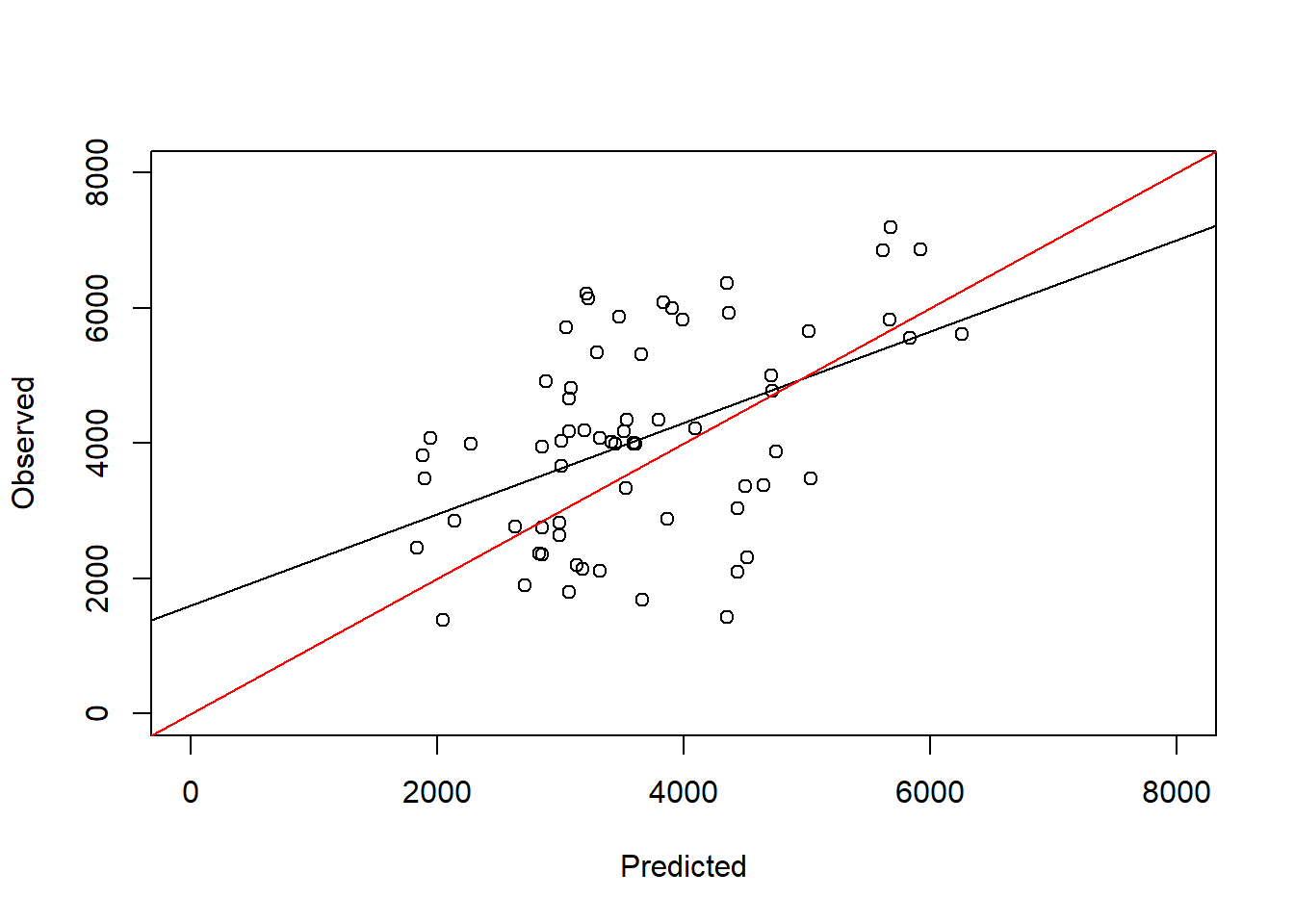
We still do not get a perfect 1:1 line, but the model is much better than the full model.
- We can redo the model selection using BIC as the criterion. We need to calculate the number of observations in the dataset and then use it in the
stepAIC()function:
n <- nrow(train_data)
step_model_bic <- stepAIC(full_model, direction = "backward", k = log(n))
Start: AIC=2363.14
maizeyield ~ EVI + precip.PC9 + precip.PC8 + precip.PC5 + precip.PC1 +
precip.PC17 + precip.PC10 + LSTD + LSTN + clyppt + drougth.days +
sltppt + cecsol + drought + taxnwrb_250m + NIR + MIR + sub_mg +
sub_k + altitude + precip.PC11
Df AIC
- precip.PC11 1 2358.3
- clyppt 1 2358.3
- sltppt 1 2358.5
- altitude 1 2358.5
- precip.PC9 1 2358.6
- sub_k 1 2358.6
- LSTN 1 2358.7
- precip.PC10 1 2358.8
- drougth.days 1 2358.8
- precip.PC1 1 2358.8
- sub_mg 1 2358.8
- precip.PC8 1 2358.8
- LSTD 1 2359.1
- cecsol 1 2359.2
- precip.PC5 1 2359.6
- NIR 1 2359.6
- precip.PC17 1 2359.7
- drought 1 2360.4
- EVI 1 2360.6
- taxnwrb_250m 1 2360.9
- MIR 1 2361.0
<none> 2363.1
Step: AIC=2358.28
maizeyield ~ EVI + precip.PC9 + precip.PC8 + precip.PC5 + precip.PC1 +
precip.PC17 + precip.PC10 + LSTD + LSTN + clyppt + drougth.days +
sltppt + cecsol + drought + taxnwrb_250m + NIR + MIR + sub_mg +
sub_k + altitude
Df AIC
- clyppt 1 2353.4
- sltppt 1 2353.6
- altitude 1 2353.7
- precip.PC9 1 2353.7
- sub_k 1 2353.8
- precip.PC1 1 2353.9
- LSTN 1 2353.9
- sub_mg 1 2353.9
- precip.PC8 1 2354.1
- drougth.days 1 2354.1
- precip.PC10 1 2354.2
- cecsol 1 2354.4
- LSTD 1 2354.5
- NIR 1 2354.8
- precip.PC17 1 2354.9
- EVI 1 2355.8
- drought 1 2355.8
- taxnwrb_250m 1 2356.1
- MIR 1 2356.2
- precip.PC5 1 2357.9
<none> 2358.3
Step: AIC=2353.45
maizeyield ~ EVI + precip.PC9 + precip.PC8 + precip.PC5 + precip.PC1 +
precip.PC17 + precip.PC10 + LSTD + LSTN + drougth.days +
sltppt + cecsol + drought + taxnwrb_250m + NIR + MIR + sub_mg +
sub_k + altitude
Df AIC
- sltppt 1 2348.8
- altitude 1 2348.8
- precip.PC9 1 2348.9
- sub_k 1 2348.9
- precip.PC1 1 2349.1
- sub_mg 1 2349.1
- LSTN 1 2349.1
- precip.PC8 1 2349.3
- drougth.days 1 2349.3
- cecsol 1 2349.5
- precip.PC10 1 2349.6
- LSTD 1 2349.7
- NIR 1 2349.9
- precip.PC17 1 2350.1
- EVI 1 2350.9
- drought 1 2351.0
- taxnwrb_250m 1 2351.3
- MIR 1 2351.4
- precip.PC5 1 2353.2
<none> 2353.4
Step: AIC=2348.76
maizeyield ~ EVI + precip.PC9 + precip.PC8 + precip.PC5 + precip.PC1 +
precip.PC17 + precip.PC10 + LSTD + LSTN + drougth.days +
cecsol + drought + taxnwrb_250m + NIR + MIR + sub_mg + sub_k +
altitude
Df AIC
- altitude 1 2344.2
- precip.PC9 1 2344.3
- sub_k 1 2344.3
- sub_mg 1 2344.3
- LSTN 1 2344.5
- precip.PC1 1 2344.6
- precip.PC8 1 2344.6
- drougth.days 1 2344.6
- cecsol 1 2344.8
- precip.PC10 1 2344.8
- LSTD 1 2345.1
- precip.PC17 1 2345.3
- NIR 1 2345.3
- EVI 1 2346.3
- drought 1 2346.4
- MIR 1 2346.6
- taxnwrb_250m 1 2346.9
- precip.PC5 1 2348.5
<none> 2348.8
Step: AIC=2344.17
maizeyield ~ EVI + precip.PC9 + precip.PC8 + precip.PC5 + precip.PC1 +
precip.PC17 + precip.PC10 + LSTD + LSTN + drougth.days +
cecsol + drought + taxnwrb_250m + NIR + MIR + sub_mg + sub_k
Df AIC
- precip.PC9 1 2339.6
- LSTN 1 2339.7
- sub_k 1 2339.7
- sub_mg 1 2339.8
- drougth.days 1 2339.8
- precip.PC1 1 2339.9
- precip.PC8 1 2339.9
- precip.PC10 1 2340.2
- cecsol 1 2340.3
- NIR 1 2340.5
- precip.PC17 1 2340.6
- LSTD 1 2340.9
- EVI 1 2341.4
- drought 1 2341.7
- MIR 1 2341.7
- taxnwrb_250m 1 2342.1
- precip.PC5 1 2343.8
<none> 2344.2
Step: AIC=2339.59
maizeyield ~ EVI + precip.PC8 + precip.PC5 + precip.PC1 + precip.PC17 +
precip.PC10 + LSTD + LSTN + drougth.days + cecsol + drought +
taxnwrb_250m + NIR + MIR + sub_mg + sub_k
Df AIC
- LSTN 1 2334.9
- sub_k 1 2335.0
- drougth.days 1 2335.1
- sub_mg 1 2335.2
- cecsol 1 2335.5
- precip.PC1 1 2335.5
- precip.PC10 1 2335.6
- NIR 1 2335.7
- precip.PC8 1 2335.8
- precip.PC17 1 2336.0
- LSTD 1 2336.1
- EVI 1 2336.6
- MIR 1 2336.9
- drought 1 2336.9
- taxnwrb_250m 1 2337.3
- precip.PC5 1 2338.9
<none> 2339.6
Step: AIC=2334.92
maizeyield ~ EVI + precip.PC8 + precip.PC5 + precip.PC1 + precip.PC17 +
precip.PC10 + LSTD + drougth.days + cecsol + drought + taxnwrb_250m +
NIR + MIR + sub_mg + sub_k
Df AIC
- sub_k 1 2330.3
- sub_mg 1 2330.6
- cecsol 1 2330.6
- drougth.days 1 2330.7
- precip.PC8 1 2330.9
- precip.PC10 1 2331.0
- NIR 1 2331.2
- LSTD 1 2331.3
- precip.PC17 1 2331.6
- precip.PC1 1 2331.7
- EVI 1 2332.2
- MIR 1 2332.5
- drought 1 2332.5
- taxnwrb_250m 1 2332.6
<none> 2334.9
- precip.PC5 1 2337.0
Step: AIC=2330.31
maizeyield ~ EVI + precip.PC8 + precip.PC5 + precip.PC1 + precip.PC17 +
precip.PC10 + LSTD + drougth.days + cecsol + drought + taxnwrb_250m +
NIR + MIR + sub_mg
Df AIC
- cecsol 1 2326.0
- drougth.days 1 2326.1
- sub_mg 1 2326.1
- precip.PC8 1 2326.3
- NIR 1 2326.6
- LSTD 1 2326.7
- precip.PC10 1 2326.7
- precip.PC17 1 2327.1
- precip.PC1 1 2327.2
- EVI 1 2327.5
- MIR 1 2327.8
- drought 1 2327.8
- taxnwrb_250m 1 2328.2
<none> 2330.3
- precip.PC5 1 2332.2
Step: AIC=2325.98
maizeyield ~ EVI + precip.PC8 + precip.PC5 + precip.PC1 + precip.PC17 +
precip.PC10 + LSTD + drougth.days + drought + taxnwrb_250m +
NIR + MIR + sub_mg
Df AIC
- drougth.days 1 2321.7
- precip.PC8 1 2321.9
- sub_mg 1 2321.9
- LSTD 1 2322.1
- NIR 1 2322.1
- precip.PC10 1 2322.2
- precip.PC17 1 2322.3
- EVI 1 2323.0
- precip.PC1 1 2323.0
- drought 1 2323.3
- taxnwrb_250m 1 2323.5
- MIR 1 2323.5
<none> 2326.0
- precip.PC5 1 2327.3
Step: AIC=2321.68
maizeyield ~ EVI + precip.PC8 + precip.PC5 + precip.PC1 + precip.PC17 +
precip.PC10 + LSTD + drought + taxnwrb_250m + NIR + MIR +
sub_mg
Df AIC
- precip.PC8 1 2317.1
- precip.PC17 1 2317.6
- sub_mg 1 2317.8
- precip.PC10 1 2317.9
- LSTD 1 2318.0
- NIR 1 2318.6
- taxnwrb_250m 1 2318.8
- MIR 1 2319.4
- drought 1 2319.4
- precip.PC1 1 2319.6
- EVI 1 2319.6
<none> 2321.7
- precip.PC5 1 2322.7
Step: AIC=2317.12
maizeyield ~ EVI + precip.PC5 + precip.PC1 + precip.PC17 + precip.PC10 +
LSTD + drought + taxnwrb_250m + NIR + MIR + sub_mg
Df AIC
- precip.PC17 1 2313.1
- precip.PC10 1 2313.2
- sub_mg 1 2313.6
- LSTD 1 2313.9
- drought 1 2314.7
- taxnwrb_250m 1 2314.7
- NIR 1 2314.9
- MIR 1 2315.1
- EVI 1 2315.5
- precip.PC1 1 2316.1
<none> 2317.1
- precip.PC5 1 2318.1
Step: AIC=2313.13
maizeyield ~ EVI + precip.PC5 + precip.PC1 + precip.PC10 + LSTD +
drought + taxnwrb_250m + NIR + MIR + sub_mg
Df AIC
- precip.PC10 1 2308.5
- sub_mg 1 2309.4
- LSTD 1 2309.7
- taxnwrb_250m 1 2310.9
- NIR 1 2311.3
- MIR 1 2312.8
- EVI 1 2312.9
- drought 1 2312.9
<none> 2313.1
- precip.PC5 1 2315.3
- precip.PC1 1 2317.2
Step: AIC=2308.48
maizeyield ~ EVI + precip.PC5 + precip.PC1 + LSTD + drought +
taxnwrb_250m + NIR + MIR + sub_mg
Df AIC
- sub_mg 1 2304.7
- LSTD 1 2305.3
- taxnwrb_250m 1 2306.1
- NIR 1 2306.8
- MIR 1 2308.1
- EVI 1 2308.2
<none> 2308.5
- drought 1 2308.5
- precip.PC5 1 2310.4
- precip.PC1 1 2313.1
Step: AIC=2304.74
maizeyield ~ EVI + precip.PC5 + precip.PC1 + LSTD + drought +
taxnwrb_250m + NIR + MIR
Df AIC
- LSTD 1 2302.0
- taxnwrb_250m 1 2302.5
- NIR 1 2303.1
- MIR 1 2304.4
- EVI 1 2304.4
- drought 1 2304.5
<none> 2304.7
- precip.PC5 1 2306.9
- precip.PC1 1 2311.5
Step: AIC=2301.98
maizeyield ~ EVI + precip.PC5 + precip.PC1 + drought + taxnwrb_250m +
NIR + MIR
Df AIC
- taxnwrb_250m 1 2299.1
- NIR 1 2299.2
- MIR 1 2300.3
- drought 1 2301.3
- EVI 1 2301.8
<none> 2302.0
- precip.PC5 1 2302.2
- precip.PC1 1 2307.9
Step: AIC=2299.06
maizeyield ~ EVI + precip.PC5 + precip.PC1 + drought + NIR +
MIR
Df AIC
- NIR 1 2296.3
- MIR 1 2297.1
- EVI 1 2297.9
<none> 2299.1
- drought 1 2299.2
- precip.PC5 1 2299.3
- precip.PC1 1 2304.5
Step: AIC=2296.35
maizeyield ~ EVI + precip.PC5 + precip.PC1 + drought + MIR
Df AIC
- MIR 1 2292.3
- EVI 1 2294.2
- drought 1 2295.2
- precip.PC5 1 2296.1
<none> 2296.3
- precip.PC1 1 2302.1
Step: AIC=2292.29
maizeyield ~ EVI + precip.PC5 + precip.PC1 + drought
Df AIC
- EVI 1 2289.3
<none> 2292.3
- precip.PC5 1 2292.4
- drought 1 2292.5
- precip.PC1 1 2298.2
Step: AIC=2289.33
maizeyield ~ precip.PC5 + precip.PC1 + drought
Df AIC
- drought 1 2287.7
- precip.PC5 1 2287.9
<none> 2289.3
- precip.PC1 1 2299.0
Step: AIC=2287.66
maizeyield ~ precip.PC5 + precip.PC1
Df AIC
- precip.PC5 1 2285.2
<none> 2287.7
- precip.PC1 1 2295.8
Step: AIC=2285.23
maizeyield ~ precip.PC1
Df AIC
<none> 2285.2
- precip.PC1 1 2293.5step_model_bicLinear mixed-effects model fit by maximum likelihood
Data: train_data
Log-likelihood: -1128.035
Fixed: maizeyield ~ precip.PC1
(Intercept)  precip.PC1
 2081.46833   -25.10853
Random effects:
Formula: ~1 | dummy
(Intercept) Residual
StdDev: 0.1022856 1610.151
Correlation Structure: corMatern
Formula: ~longitude + latitude | dummy
Parameter estimate(s):
range nu
0.02074149 0.12448933
Number of Observations: 129
Number of Groups: 1 We can see that the model selected by BIC is different from the one selected by AIC. In fact, the model selected by BIC only has one predictor (precip.PC1):
step_model$coef$fixed (Intercept) EVI precip.PC5 precip.PC1 LSTD drought
2442.699605 2.504254 -54.419094 -24.515219 -136.640292 940.701870
taxnwrb_250m NIR MIR
8.429614 -4.109523 3.831153 step_model_bic$coef$fixed(Intercept) precip.PC1
2081.46833 -25.10853 This is a good example of how the choice of information criterion can affect the model. The AIC of the best BIC model is actually not very different from the best AIC model:
AIC(step_model)[1] 2267.567AIC(step_model_bic)[1] 2268.071But the BICs are:
BIC(step_model)[1] 2304.744BIC(step_model_bic)[1] 2285.23Let’s evaluate the performance of the best BIC model in the test dataset:
pred_step_bic <- predict(step_model_bic, newdata = test_data)
rmse_step_bic <- sqrt(mean((test_data$maizeyield - pred_step_bic)^2))
c(rmse_step_bic, rmse_step)
[1] 1387.247 1410.906It actually performs better than the best AIC model. If we take predictive RMSE as the best performance metric, then one would conclude that BIC was a better criterion for model selection in this case. If we model the relationship between observed and predicted values:
eval_step_bic <- lm(test_data$maizeyield~pred_step_bic)
summary(eval_step_bic)
Call:
lm(formula = test_data$maizeyield ~ pred_step_bic)

Residuals:
    Min      1Q  Median      3Q     Max
-3335.8  -926.5   -70.7  1071.9  2233.1

Coefficients:
               Estimate Std. Error t value Pr(>|t|)
(Intercept)   1257.2660   682.7175   1.842   0.0701 .
pred_step_bic    0.7688     0.1815   4.236 7.32e-05 ***
---
Signif. codes:  0 '***' 0.001 '**' 0.01 '*' 0.05 '.' 0.1 ' ' 1

Residual standard error: 1328 on 65 degrees of freedom
Multiple R-squared:  0.2163,    Adjusted R-squared:  0.2043
F-statistic: 17.95 on 1 and 65 DF, p-value: 7.315e-05plot(test_data$maizeyield~pred_step_bic, ylab = "Observed", xlab = "Predicted",
xlim = c(0, 8e3), ylim = c(0, 8e3))
abline(eval_step_bic)
abline(a = 0, b = 1, col = "red")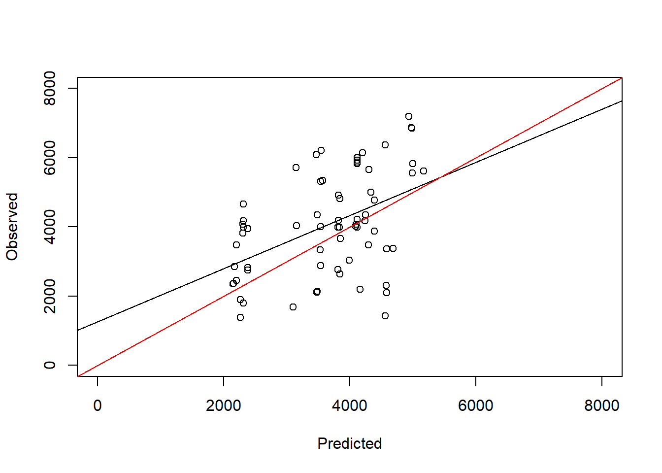
We can see that in this model the slope is closer to 1 and the intercept is closer to 0 compared to the best AIC model.
10.2 Cross-validation to evaluate model performance
As show in the previous section, one can use information criteria to select the best model from a set of candidate models. However, this approach has some limitations and it is not clear a priori which criterion is going to work better with a given dataset a model. As hinted in the exercise, RMSE calculated on a test dataset is a better metric to evaluate the performance of a model. For that reason, an alternative to information criteria is to use cross-validation. Cross-validation is a technique that splits the dataset into a training and a test set multiple times and then evaluates the performance of the model in the test set. This allows us to get a more robust estimate of the performance of the model.
First, let’s join the two datasets we loaded before, as we will let the algorithm select which subsets to use for training and testing:
all_data <- rbind(train_data, test_data)We are also going to add something to the model. We are going to create a new variable that represents geographical clusters of the data (like regions). We can see this clustering in the data by plotting the locations of the data:
with(all_data, plot(longitude, latitude))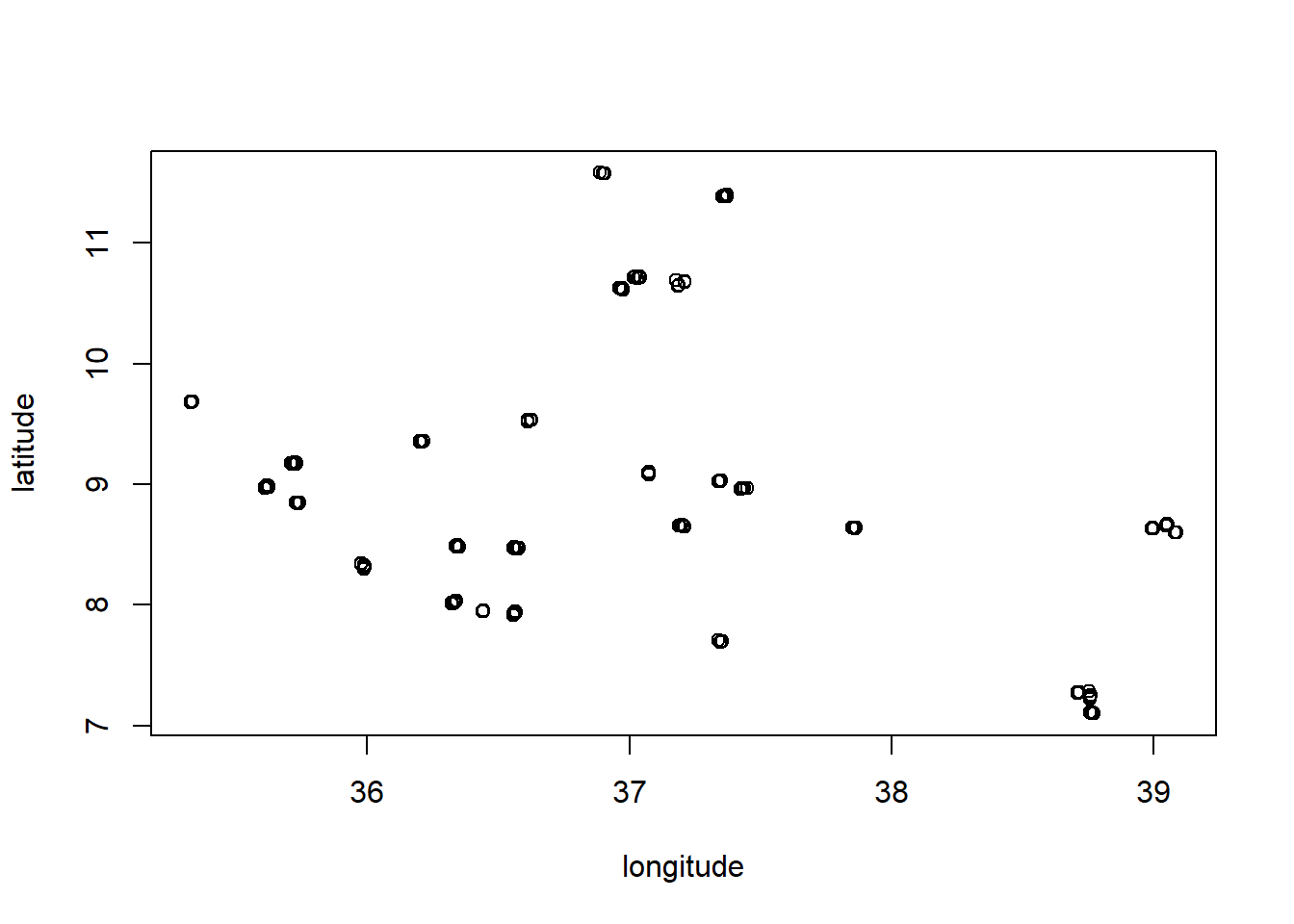
We can see that there are some clear clusters in the data. We can create a new variable that represents these clusters by using the kmeans() function. This will distribute the data into a specified number of clusters (we choose 10) based on the geographical coordinates:
clust <- kmeans(as.matrix(all_data[,c("longitude","latitude")]), centers = 10)
all_data$cluster <- factor(clust$cluster)
We can now redo the plot of the data with the cluster numbers on top of it:
colors <- rainbow(nlevels(all_data$cluster))
with(all_data, plot(longitude, latitude, col = colors[cluster], cex = 0.5))
text(clust$centers, labels = 1:length(colors), col = "black", offset = 0)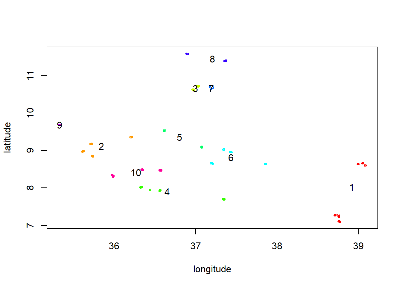
Let’s use the best AIC model but now fit it to the whole dataset using dummy as the random effect or cluster:
lmm.0 <- lme(maizeyield ~ EVI + precip.PC5 + precip.PC1 + LSTD + drought + taxnwrb_250m +
                          NIR + MIR,
            random = ~ 1 | dummy,
            correlation = corMatern(form = ~ longitude+latitude | dummy),
            data = all_data)
lmm.1 <- lme(maizeyield ~ EVI + precip.PC5 + precip.PC1 + LSTD + drought + taxnwrb_250m +
                          NIR + MIR,
            random = ~ 1 | cluster,
            correlation = corMatern(form = ~ longitude+latitude | cluster),
            data = all_data)
anova(lmm.0, lmm.1)
Model df AIC BIC logLik
lmm.0 1 13 3350.383 3392.388 -1662.192
lmm.1 2 13 3350.352 3392.356 -1662.176We can see that there is virtually no difference. We could not evaluate the predict performance of the new model by doing 10-fold cross-validation using predictive RMSE as criterion. We can implement this with the cv() function from the cv package:
library(cv)Warning: package 'cv' was built under R version 4.4.1Loading required package: doParallelWarning: package 'doParallel' was built under R version 4.4.1Loading required package: foreachWarning: package 'foreach' was built under R version 4.4.1Loading required package: iteratorsWarning: package 'iterators' was built under R version 4.4.1Loading required package: parallelcv.res <- cv(lmm.1, k = 10, criterion = rmse, seed=123)R RNG seed set to 123Exercise 10.2
- Compare the cross-validation RMSE of the best AIC model with the RMSE of the best AIC model in the original test dataset (calculated in previous exercise).
- Perform cross-validation on the model with clusters by setting
clusterVariables="cluster"and compare with the cross-validation above.
Solution 10.2
- Let’s compare the cross-validation RMSE (an average of 10 test sets) with the RMSE calculated before:
# RMSE of the best AIC model in cross-validation
cv.res
10-Fold Cross Validation
criterion: rmse
cross-validation criterion = 1480.613
full-sample criterion = 1410.146 # RMSE of the best AIC model in the orignal test dataset
pred_step <- predict(step_model, newdata = test_data)
rmse_step <- sqrt(mean((test_data$maizeyield - pred_step)^2))
rmse_step[1] 1410.906We can see that the RMSE of the cross-validation is similar to the RMSE of the test dataset but not the same. Averaging over multiple possible train-set split is important due to variation across samples (both for training and testing).
- We can perform cross-validation on the model with clusters by making sure that all the data from a cluster is either in the train or the test dataset:
cv.res.cluster <- cv(lmm.1, k = 10, criterion = rmse, clusterVariables="cluster", seed=123)Note: seed ignored for n-fold CVcv.res.clustern-Fold Cross Validation based on 10 {cluster} clusters
criterion: rmse
cross-validation criterion = 1747.104
full-sample criterion = 1427.435 The RMSE is now much larger. The reason is that in the previous setup, the random effect of a cluster could be used to predict the yield within the same cluster in the test dataset. In this setup, the model is forced to predict yields in clusters that it has not seen before which of course results in worse predictive performance. Whether we should be using this approach or the previous one depends on the goals of the prediction task.
10.3 Simulating nested data
In this final exercise we will simulate nested data. We will simulate a dataset with a nested structure of two levels (B within A) and three replicates:
n.lev.A <- 10
n.lev.B <- 5
n.obs <- 3
design <- expand.grid(A = factor(1:n.lev.A),
                      B = factor(1:n.lev.B),
                      obs = factor(1:n.obs))
design <- design[with(design, order(A, B, obs)),]
Add two covariates of interest, x1 and x2 that are independent of each other:
set.seed(1234)
design$x1 <- rnorm(nrow(design), mean = 0, sd = 5)
design$x2 <- rnorm(nrow(design), mean = 0, sd = 5)
Let’s now create the matrices of fixed and random effects (for the latter we use the function getMM from the VCA package):
library(VCA)Warning: package 'VCA' was built under R version 4.4.1
Attaching package: 'VCA'The following objects are masked from 'package:spaMM':
fixef, ranefThe following objects are masked from 'package:nlme':
fixef, isBalanced, raneflibrary(lmerTest)Loading required package: lme4Loading required package: Matrix
Attaching package: 'lme4'The following objects are masked from 'package:VCA':
fixef, getL, ranefThe following object is masked from 'package:nlme':
lmList
Attaching package: 'lmerTest'The following object is masked from 'package:lme4':
lmerThe following object is masked from 'package:stats':
stepX <- as.matrix(design[,c("x1","x2")], ncol = 2)
Z <- getMM(~A/B-1, Data = design)We can create the vector of coefficients:
Beta <- matrix(c(0.1, 0.22), ncol = 1)And the covariance matrix of the random effects:
sigma_A <- 100^2 # random effect A variance
sigma_B <- 200^2 # random effect B variance
sigma <- 50^2 # residual variance
# Covariance matrix of random effects
G <- diag(c(rep(sigma_A,n.lev.A), rep(sigma_B,n.lev.B*n.lev.A)))
ZGTZ <- Z%*%G%*%t(Z)
# Covariance matrix of residuals
R <- diag(sigma,nrow(design))
V <- ZGTZ + R
Finally we can simulate some data:
set.seed(123)
library(mvtnorm)
design$y <- c(rmvnorm(1,mean = c(X%*%Beta), sigma = as.matrix(V)))
Exercise 10.3
- Visualize the matrices using
image()and discuss them in the context of the structure of the data. - Fit a linear mixed model to the data using
lmer()from thelme4package (check above for the model formulae). Compare the estimates to the true values. - Fit a second model ignoring the factor
B. Compare to the previous model and show which is one is better.
Solution 10.3
- We can visualize the matrices using
image():
image(V)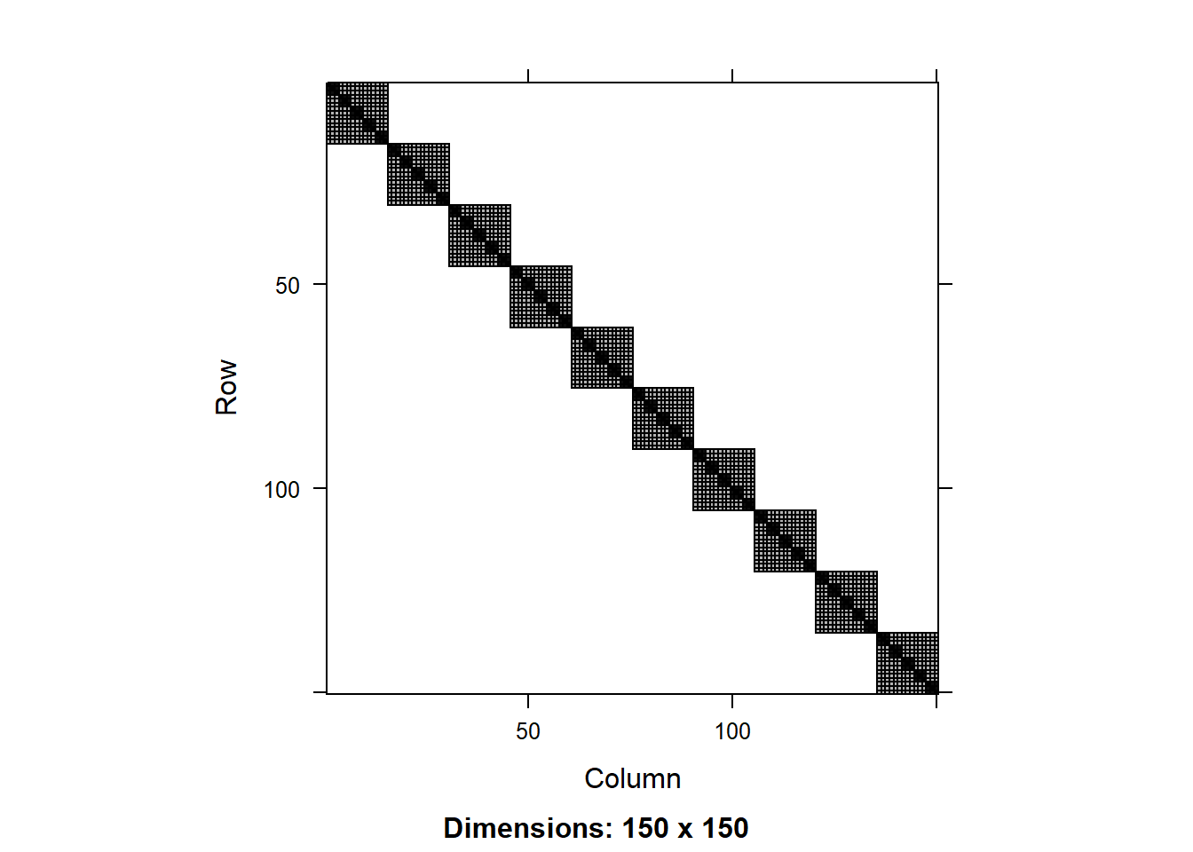
image(R)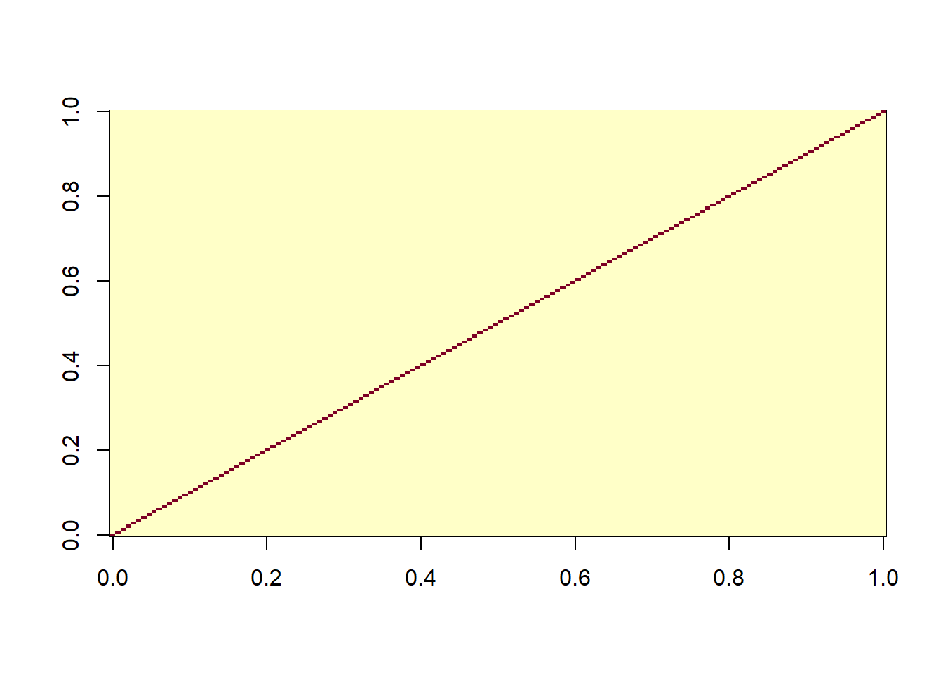
The matrix of residuals is a simple diagonal matrix, which makes sense as we have assumed that the residuals are independent. The matrix of the full model shows the nested structure of the data.
- We can fit the linear mixed model to the data:
lmm1 <- lmer(y ~ x1 + x2 - 1 + (1|A/B), data = design)
summary(lmm1)
Linear mixed model fit by REML. t-tests use Satterthwaite's method [
lmerModLmerTest]
Formula: y ~ x1 + x2 - 1 + (1 | A/B)
Data: design
REML criterion at convergence: 1778.8
Scaled residuals:
Min 1Q Median 3Q Max
-2.11653 -0.53546 -0.04726 0.47151 2.31239
Random effects:
Groups Name Variance Std.Dev.
B:A (Intercept) 32849 181.24
A (Intercept) 5663 75.25
Residual 2360 48.58
Number of obs: 150, groups: B:A, 50; A, 10
Fixed effects:
Estimate Std. Error df t value Pr(>|t|)
x1 0.8579 1.0740 100.7810 0.799 0.426
x2 1.5585 0.9511 100.4698 1.639 0.104
Correlation of Fixed Effects:
x1
x2 0.090The true values for the coefficients were 0.1 and 0.22 but the model estimates are much larger, but still in the right ballpark. In fact, both estimates are not significantly different from zero (or the true values for that matter). The variance of the residual is well estimated and close to the true value, but the variance of the random effects are underestimated (the true values were 40,000 and 10,000 but the estimated values were 32,849 and 5,663, respectively).
- We can fit a second model ignoring the factor
B:
lmm2 <- lmer(y ~ x1 + x2 - 1 + (1|A), data = design)
summary(lmm2)
Linear mixed model fit by REML. t-tests use Satterthwaite's method [
lmerModLmerTest]
Formula: y ~ x1 + x2 - 1 + (1 | A)
Data: design
REML criterion at convergence: 1983.4
Scaled residuals:
Min 1Q Median 3Q Max
-2.30492 -0.84022 0.07432 0.68020 2.23808
Random effects:
Groups Name Variance Std.Dev.
A (Intercept) 10341 101.7
Residual 30686 175.2
Number of obs: 150, groups: A, 10
Fixed effects:
Estimate Std. Error df t value Pr(>|t|)
x1 -0.3279 3.1700 144.1078 -0.103 0.918
x2 4.0954 2.8149 140.5208 1.455 0.148
Correlation of Fixed Effects:
x1
x2 0.066We can ssee that the variance of the residual is significantly larger than the true value, while the variance of the random effect of A is quite similar to the true value. We can compare the two models using the AIC or using the likelihood ratio test:
anova(lmm1, lmm2)refitting model(s) with ML (instead of REML)Data: design
Models:
lmm2: y ~ x1 + x2 - 1 + (1 | A)
lmm1: y ~ x1 + x2 - 1 + (1 | A/B)
npar AIC BIC logLik deviance Chisq Df Pr(>Chisq)
lmm2 4 1999.4 2011.5 -995.70 1991.4
lmm1 5 1792.5 1807.6 -891.26 1782.5 208.89 1 < 2.2e-16 ***
---
Signif. codes: 0 '***' 0.001 '**' 0.01 '*' 0.05 '.' 0.1 ' ' 1With both criteria it is clear that the model that includes the factor B is much better (as expected).
Let’s simulate some new data from the two models fitted in the exercise:
sim.values.1 <- simulate(lmm1, nsim = 1000, seed = 123)
sim.values.2 <- simulate(lmm2, nsim = 1000, seed = 124)
We can make a nice visualization:
cols <- rainbow(nlevels(design$A))
pchs <- c(21:25)

par(mfrow=c(3,1))
with(design,plot(y,col=cols[A],pch=pchs[B]))
with(design,plot(sim.values.1[,1],col=cols[A],pch=pchs[B]))
with(design,plot(sim.values.2[,2],col=cols[A],pch=pchs[B]))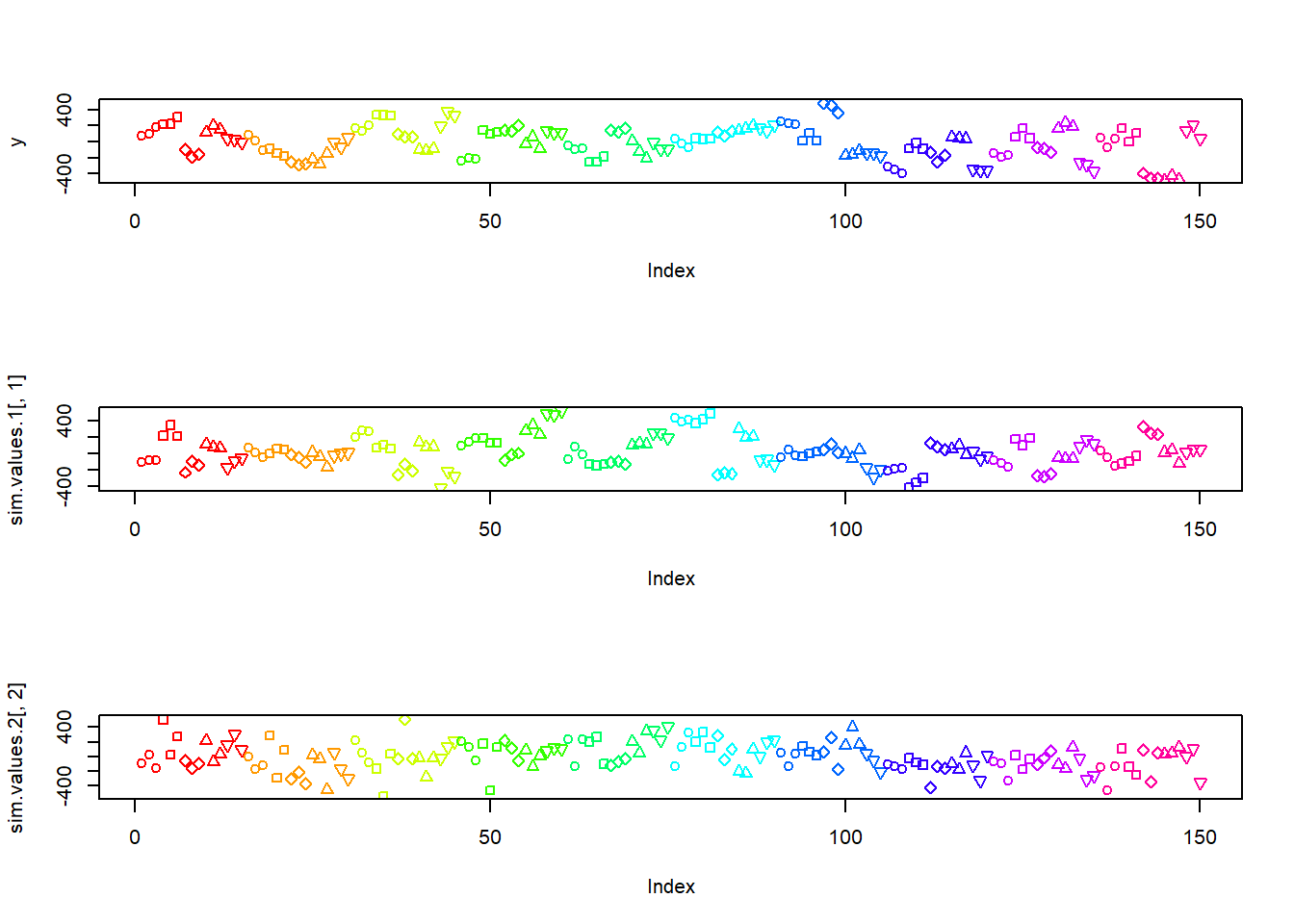
par(mfrow = c(1,1))Let’s fit the true model to both datasets:
lmm1.sim <- lmer(sim.values.1[,1] ~ x1 + x2 - 1 + (1|A/B), data = design)
lmm2.sim <- lmer(sim.values.2[,1] ~ x1 + x2 - 1 + (1|A/B), data = design)
Exercise 10.4
- Check the estimates of the fixed and random effects of
lmm1.simandlmm2.sim.
Solution 10.4
- We can check the estimates of the fixed and random effects of
lmm1.simandlmm2.sim:
summary(lmm1.sim)Linear mixed model fit by REML. t-tests use Satterthwaite's method [
lmerModLmerTest]
Formula: sim.values.1[, 1] ~ x1 + x2 - 1 + (1 | A/B)
Data: design
REML criterion at convergence: 1782.1
Scaled residuals:
Min 1Q Median 3Q Max
-2.24327 -0.50124 0.02161 0.59865 1.82023
Random effects:
Groups Name Variance Std.Dev.
B:A (Intercept) 32816 181.15
A (Intercept) 1150 33.91
Residual 2553 50.53
Number of obs: 150, groups: B:A, 50; A, 10
Fixed effects:
Estimate Std. Error df t value Pr(>|t|)
x1 0.5887 1.1154 101.3633 0.528 0.5988
x2 1.8455 0.9883 100.8048 1.867 0.0648 .
---
Signif. codes: 0 '***' 0.001 '**' 0.01 '*' 0.05 '.' 0.1 ' ' 1
Correlation of Fixed Effects:
x1
x2 0.089summary(lmm2.sim)Linear mixed model fit by REML. t-tests use Satterthwaite's method [
lmerModLmerTest]
Formula: sim.values.1[, 2] ~ x1 + x2 - 1 + (1 | A/B)
Data: design
REML criterion at convergence: 1768.3
Scaled residuals:
Min 1Q Median 3Q Max
-2.02577 -0.62875 0.01437 0.52634 1.68805
Random effects:
Groups Name Variance Std.Dev.
B:A (Intercept) 26942 164.14
A (Intercept) 0 0.00
Residual 2487 49.87
Number of obs: 150, groups: B:A, 50; A, 10
Fixed effects:
Estimate Std. Error df t value Pr(>|t|)
x1 1.048 1.099 102.198 0.954 0.342
x2 -0.091 0.974 101.409 -0.093 0.926
Correlation of Fixed Effects:
x1
x2 0.089
optimizer (nloptwrap) convergence code: 0 (OK)
boundary (singular) fit: see help('isSingular')The results from the first model (lmm1.sim) are similar to the ones obtained in the previous exercise. Although the exact values are different because of sample variability. In the second model (lmm2.sim) we observed that the variance for the random effect of A is extactly 0 (and we got a warning message regarding singularity when fitting). This is because the simulated data was generated without the random effect of B, so the model cannot estimate the random effect of A and B properly. In this case, the model estimated the variance from the lower level of the hierarchy (B:A).