# Covariance matrix that combines random effects and residual (V = ZGZ^t + R)
getV <- function(model) {
  Lamda<-getME(model,"Lambda") ##matrix with scaling factor for random sd (relative to sigma)
  var.lamda <- t(Lamda)%*%Lamda ## scale for variance (sigma^2)
  Z <- getME(model,"Z")
  sigma2 <- sigma(model)^2 ##
  var.g<-sigma2*var.lamda
  var.random <- (Z %*% var.g %*%t(Z))
  var.resid <- sigma2 *Diagonal(nrow(Z))
  var.y <- var.random + var.resid
  invisible(var.y)
}6 Linear mixed models III
6.1 Auxiliary functions
We will use the following function to extract the covariance matrix of a linear mixed model:
6.2 Random regression with uncorrelated random intercepts and slopes
Let’s simulate some data where the slopes of a regression line vary across groups. We will assumme a quantitative predictor (Irrigation) and its effect on yield across different locations:
Irrigation <- c(0,250,500,750,1000) # levels of irrigation (mm)
location <- factor(1:16)
design <- expand.grid(Irrigation = Irrigation, location = location)
Estimating intercepts and slopes simulatenously can be difficult because these two parameters tend to be correlated. We can reduce this correlation by centering the predictor variable:
design$Irrigation.ct <- scale(design$Irrigation, scale = FALSE)This means that the intercept of a model using Irrigation.ct corresponds to the response when Irrigation is average and not zero. Let’s make the mixed effect model and simulate some data:
library(designr) # For the function simLMM()
mixef.form <- ~ Irrigation.ct + (Irrigation.ct|location)
Fixef <- c(2000,10) # Intercept and slope
VC_sd <- list(c(200,10), 300) # standard deviation of random intercept, slope and residual\
set.seed(123)
design$y <- simLMM(formula = mixef.form, CP = 0.0, data = design, Fixef = Fixef,
                   VC_sd = VC_sd)
Data simulation from a linear mixed-effects model (LMM)
Formula: gaussian ~ 1 + Irrigation.ct + ( 1 + Irrigation.ct | location )
empirical = FALSE
Random effects:
Groups Name Std.Dev. Corr
location (Intercept) 200.0
Irrigation.ct 10.0 0.00
Residual 300.0
Number of obs: 80, groups: location, 16
Fixed effects:
(Intercept) Irrigation.ct
2000 10 Let’s visualize the data. We will use the ggplot2 package for its facetting capabilities. We plot the relationship between Irrigation and y for each location and draw a linear model fitted to the data for each location (this is used as a visual reference, these are not predictions from a model!):
library(ggplot2)
ggplot(design, aes(x = Irrigation, y = y)) +
  geom_point() +
  geom_smooth(method = "lm", se = FALSE, col = "lightgray", lty = 2) +
  facet_wrap(~location) +
  theme_bw()
`geom_smooth()` using formula = 'y ~ x'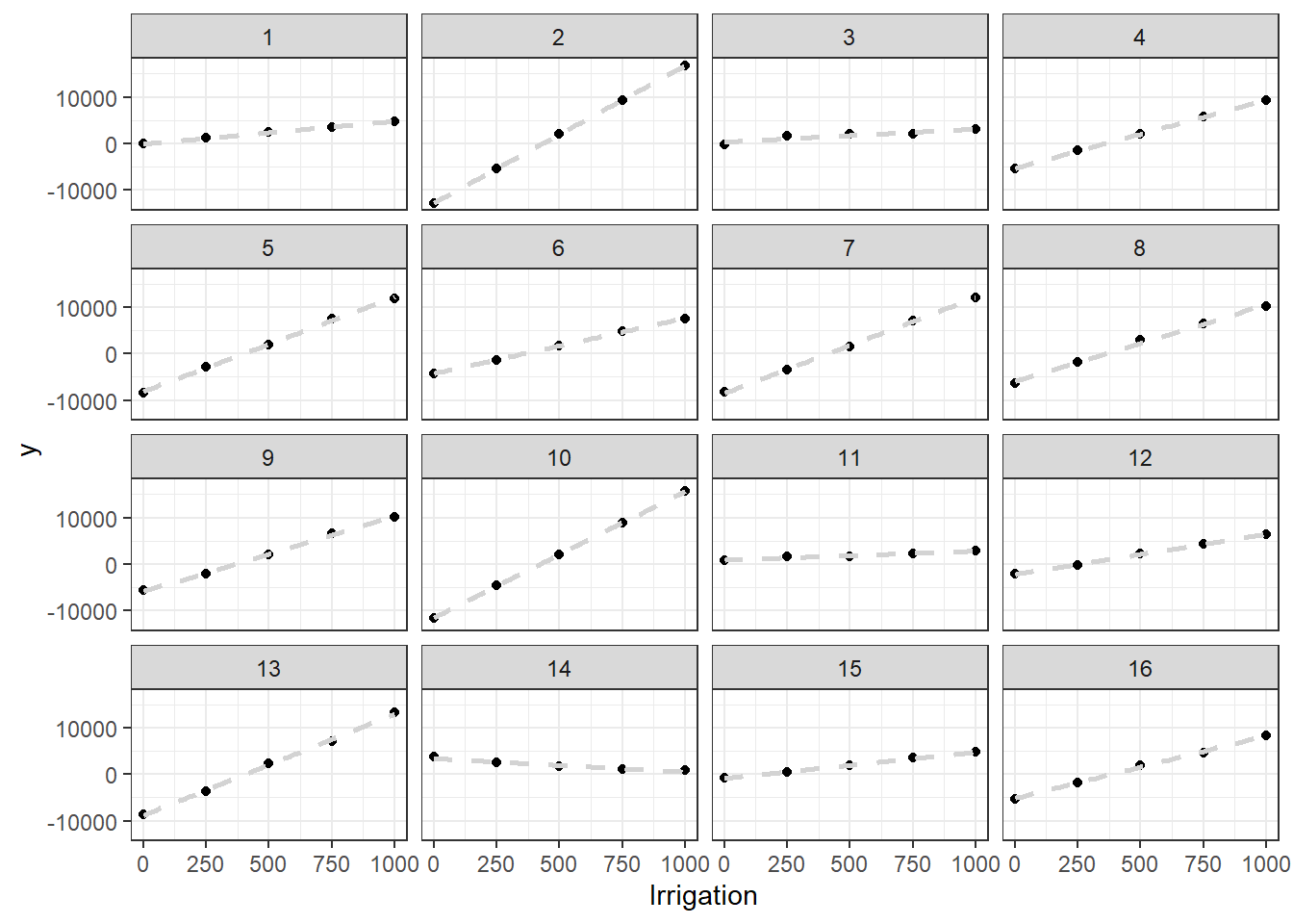
In previous chapters we computed marginal means using emmeans(). For slopes, we can use the similar function emtrends() from the same package. Let’s fit a linear model to the data to served as example:
library(emmeans)Welcome to emmeans.
Caution: You lose important information if you filter this package's results.
See '? untidy'lm1 <- lm(y~location*Irrigation.ct, data = design)
emt <- emtrends(lm1, ~ 1, var = "Irrigation.ct")
emt 1 Irrigation.ct.trend SE df lower.CL upper.CL
overall 13.3 0.0865 48 13.2 13.5
Results are averaged over the levels of: location
Confidence level used: 0.95 This function is averaging the estimates and standard errors of slopes across the different locations, that is, it is giving an estimate of the average slope.
Alternatively, we can fit a linear mixed model where we treat location as a random effect and we vary both the intercepts and the slopes across locations (the || operator is used to specify that the random effects for the intercept and the slope are assumed independent):
library(lme4)Loading required package: Matrixlibrary(lmerTest)
Attaching package: 'lmerTest'The following object is masked from 'package:lme4':
lmerThe following object is masked from 'package:stats':
steplmm1 <- lmer(y ~ Irrigation.ct + (Irrigation.ct || location), data = design)Warning in checkConv(attr(opt, "derivs"), opt$par, ctrl = control$checkConv, :
Model failed to converge with max|grad| = 0.0054334 (tol = 0.002, component 1)summary(lmm1)Linear mixed model fit by REML. t-tests use Satterthwaite's method [
lmerModLmerTest]
Formula: y ~ Irrigation.ct + (Irrigation.ct || location)
Data: design
REML criterion at convergence: 1231.6
Scaled residuals:
Min 1Q Median 3Q Max
-2.15888 -0.56877 -0.00966 0.51580 2.58137
Random effects:
Groups Name Variance Std.Dev.
location (Intercept) 26938.66 164.130
location.1 Irrigation.ct 87.25 9.341
Residual 74877.78 273.638
Number of obs: 80, groups: location, 16
Fixed effects:
Estimate Std. Error df t value Pr(>|t|)
(Intercept) 1973.078 51.182 14.994 38.550 < 2e-16 ***
Irrigation.ct 13.347 2.337 14.997 5.712 4.12e-05 ***
---
Signif. codes: 0 '***' 0.001 '**' 0.01 '*' 0.05 '.' 0.1 ' ' 1
Correlation of Fixed Effects:
(Intr)
Irrigatn.ct 0.000
optimizer (nloptwrap) convergence code: 0 (OK)
Model failed to converge with max|grad| = 0.0054334 (tol = 0.002, component 1)We can see that the estimate of the average slope is the same whether we calculate the marginal slope from the linear model or the slope from the linear mixed model. However, the standard error of the slope is much larger for the linear mixed model. Let’s repeat the previous plot but now with the slopes estimated by the linear mixed model:
design$pred<-predict(lmm1)
library(ggplot2)
ggplot(design, aes(x = Irrigation.ct, y = y)) +
  geom_point() +
  geom_line(aes(x= Irrigation.ct, y= pred),color="blue") +
  geom_smooth(method = "lm", se = FALSE, col = "lightgray", lty = 2) +
  facet_wrap(~location) +
  theme_bw()
`geom_smooth()` using formula = 'y ~ x'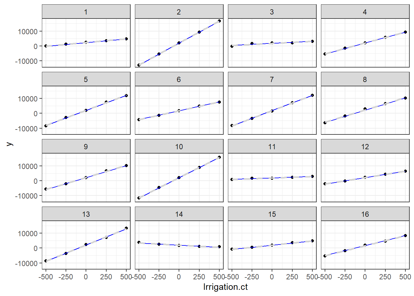
Note that we do not see much evidence of shrinkage in the slopes or intercepts (the estimated intercepts and slopes for each location are practically the same as when you fit a separate linear model to each location). The two models seem to fit the data in a very similar way. However, as usual, ignoring the structure of the data leads to very different estimations of uncertainty.
We have already stated in several chapters that ignoring the structure of the data by fitting naive linear models leads to an underestimation of uncertainty. Rather than accepting this dogmatically we demonstrate below that this is indeed the case. We generate multiple possible samples from the same model used above and fit a linear model to each of them:
n.sim <- 1000 # number of simulations
Ir.coef.sim.vec <- numeric(n.sim) # vector to store the slope estimates
for(i in 1: n.sim) {
    # Generate a new sample
    y.sim <- simLMM(formula = mixef.form, CP = 0.0, data = design, Fixef = Fixef,
                    VC_sd = VC_sd, verbose = F)
    # fit simple linear model
    lm0.sim <- lm(y.sim ~ Irrigation.ct, data = design)
    # Store the corresponding slope estimate
    Ir.coef.sim.vec[i] <- coef(lm0.sim)["Irrigation.ct"]
}
We can visualize the distribution of the slope estimates across the different models:
hist(Ir.coef.sim.vec, breaks = 20,  freq = F, xlab = "simulatedcoefficient",main="")
abline(v= Fixef[2], col = "blue", lty = 2, lwd = 2) # True value of the slope
abline(v= mean(Ir.coef.sim.vec), col = "green", lty = 2, lwd = 2) # Mean of the estimates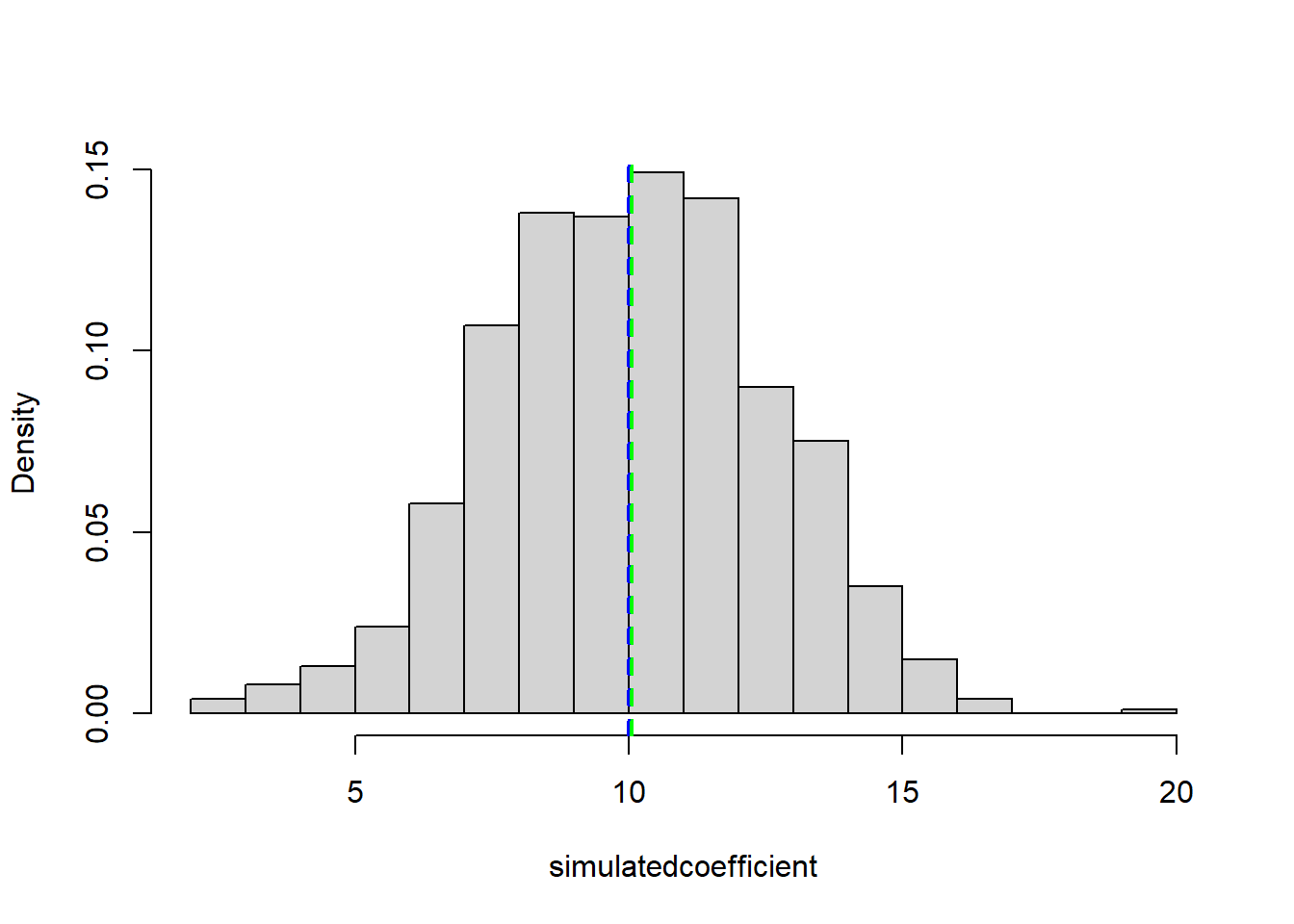
We can see that the distribution of the slope estimates is centered around the true value of the slope (blue dashed line). This means that the estimates of the slopes are unbiased. Let’s compare the standard deviation of the estimates across different samples with the standard from the linear model and the linear mixed model:
c(sim = sd(Ir.coef.sim.vec),
  lm = summary(lm1)$coefficients["Irrigation.ct", "Std. Error"],
  lmm = summary(lmm1)$coefficients["Irrigation.ct", "Std. Error"])
sim lm lmm
2.5197040 0.3461534 2.3367998 We can see that the standard error from the linear model is much smaller than the actual standard deviation across replicates (about 8 times smaller). This mismatch happens because the linear model differs from the true model underlying the data. Of course, in practice, there is no true model underlying observed data but accounting for the structure of the data brings us closer to the truth.
Exercise 6.1
Extract the covariance matrix, visualize it and explain the different components in relation to the data structure.
Extract the different values from the matrix (diagonal and off-diagonal values) and show how these values can be calculated from the variances reported in the summary of the model.
Solution 6.1
- We can use the
getV()function provided above to extract the covariance matrix of the linear mixed model:
V = getV(lmm1)
image(V)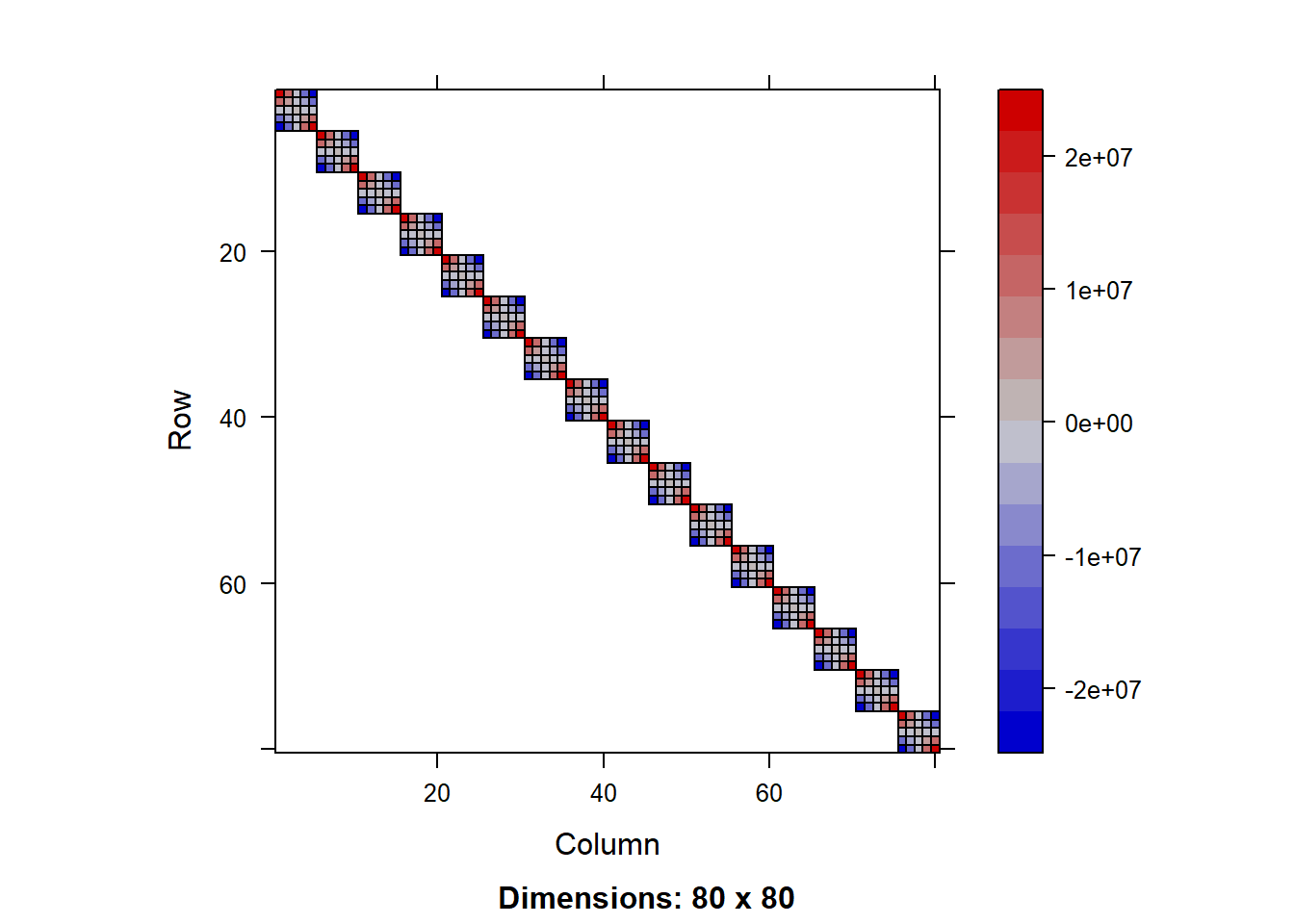
We can see that the covariance matrix has blocks of 5x5 observations, corresponding to the 5 levels of irrigation in each location. We can see different colors along the diagonal, indicating that the variance of the residuals is different for each irrigation level, being largest as one moves away from the mean irrigation level. This is typical of linear regression where uncertainty is minimal at the mean of the predictor variable and increases as we move away from it. Similarly, the covariation between and observation and other observations in the same group decreases from a strong positive correlation towards a strong negative correlation as one moves away in irrigation levels. Interestingly, the observation at the mean predictor has very little correlation with other observations (grey shade) and that is a consequence of centering the predictor (i.e., that observation is equal to the intercept of the model).
- All non-zero values in the covariance matrix are in blocks of 5x5 observations, so we can just look at the first block to see the values:
V[1:5, 1:5]5 x 5 sparse Matrix of class "dgCMatrix"
1 2 3 4 5
1 21914398.23 10933229.56 26938.66 -10879352.23 -21785643.13
2 10933229.56 5554961.89 26938.66 -5426206.79 -10879352.23
3 26938.66 26938.66 101816.44 26938.66 26938.66
4 -10879352.23 -5426206.79 26938.66 5554961.89 10933229.56
5 -21785643.13 -10879352.23 26938.66 10933229.56 21914398.23The total variances are the diagonal values:
diag(V[1:5, 1:5]) 1 2 3 4 5
21914398.2 5554961.9 101816.4 5554961.9 21914398.2 The variances reported in the summary of the model are as follows (from summary(lmm1)):
- intercept variance: 26938.66
- slope variance: 87.25
- residual variance: 74877.78
Note that these numbers are actually truncated to 2 decimal places and since the values of the variance-covariance matrix are very large numbers we actually need to use more exact values of these variances to make the calculations match. We can extract the exact values of the variances in the summary using the VarCorr() function:
vars_model = as.data.frame(VarCorr(lmm1))
vars_model
grp var1 var2 vcov sdcor
1 location (Intercept) <NA> 26938.66299 164.130019
2 location.1 Irrigation.ct <NA> 87.25033 9.340788
3 Residual <NA> <NA> 74877.77587 273.638038The column vcov is the one that contains the variance components:
vars <- vars_model$vcov # intercept, slope and residual variancesThe variance for Irrigation.ct = 0 should be the variance of intercept plus the residual variance and this should correspond to the third diagonal value in the covariance matrix:
vars[1] + vars[3] - V[3,3][1] 0The covariance for between observations at Irrigation.ct = 0 and other observations should be equal to the variance of the intercept. This corresponds to the “grey crosses” in the matrix image (row and columns 3 in the first 5x5 block):
V[c(1,2,4,5),3] == V[3,c(1,2,4,5)] 1 2 4 5
TRUE TRUE TRUE TRUE V[1,3] - vars[1][1] 0So far so great, the difficulty now comes when we look at the diagonal or off-diagonal values for other irrigation levels. This difficulty is introduced by the use of continuous covariates. From the initial lectures, you may remember that the variance of a constant times a random variable is equal to the constant squared times the variance of the random variable. This translates to models with covariates:
unique(design$Irrigation.ct) [,1]
[1,] -500
[2,] -250
[3,] 0
[4,] 250
[5,] 500fixef(lmm1) (Intercept) Irrigation.ct
1973.07820 13.34676 The total variance for observations at Irrigation.ct = 250 should be the variance of the intercept plus the residual variance plus the slope variance scaled by the squared of Irrigation.ct (we saw a similar example in the lecture):
V[2,2] - (vars[1] + vars[3] + 250^2*vars[2])[1] 1.862645e-09For the covariance terms between observations we should use the variance of the intercept plus the produce of the slope variance and the values of Irrigation.ct:
V[1,2] - (vars[1] + 500*250*vars[2])[1] 3.72529e-09A diagnostic plot specific for linear mixed models is the so-called zeta profile plot. This is a way of visualizing the confidence intervals of each coefficient in the model. In such plots, a linear relationship between the zeta profile parameter and the values of the coefficient implies that the theory used to estimate standard errors holds exactly (technically it means that the likelihood profile for that coefficient is a quadratic function). Strong deviations from linearity implies deviations from theory and therefore the standard errors may not be reliable. We can generate these profiles as follows:
library(lattice) # for xyplot
pr01 <- profile(lmm1)
xyplot(pr01, aspect = 1.3)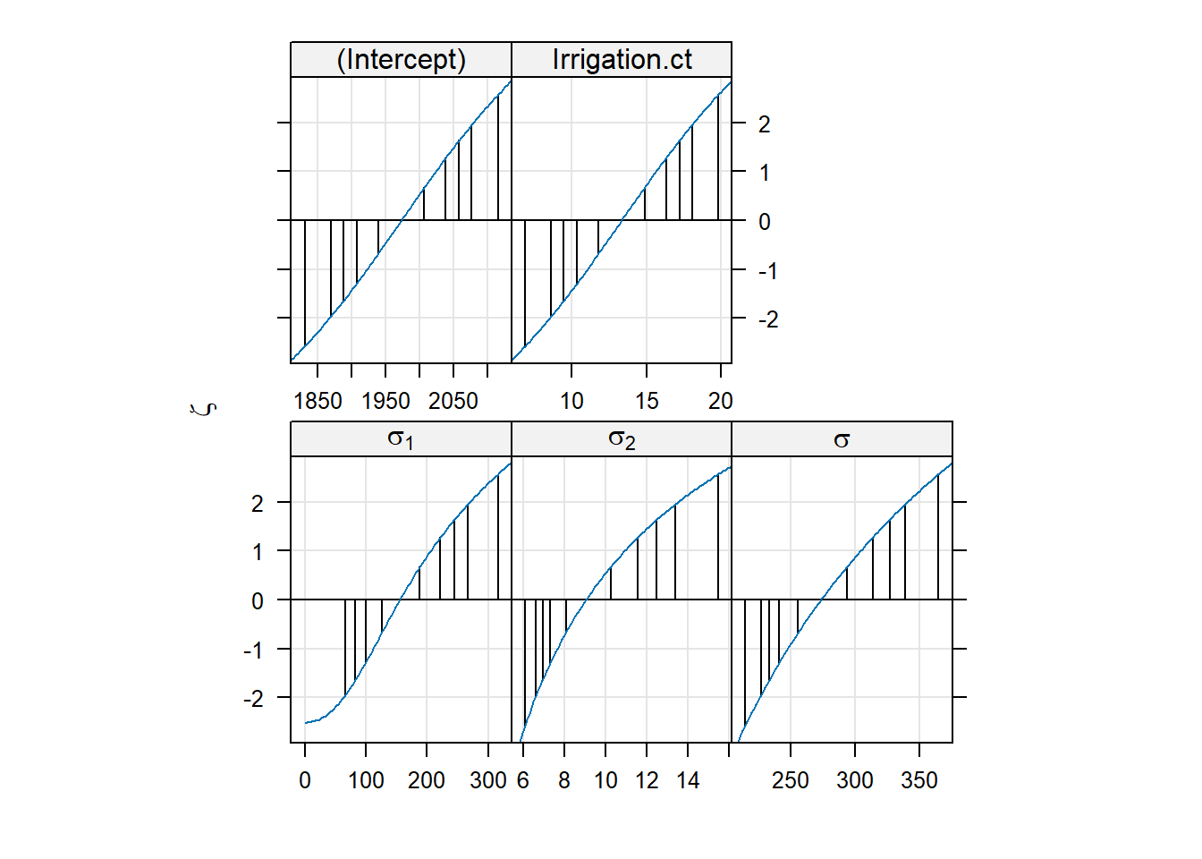
These are reasonable plots, although for some coefficients there is some curvature.
6.3 Random regression with correlated random intercepts and slopes
We now simulate the same data as before but now we assume that the random intercepts and slopes are correlated. We can do this by setting CP within simLMM() to a value different from zero:
set.seed(123)
design$y.cor <- simLMM(formula= mixef.form, CP = -0.25, data = design, Fixef = Fixef,
                       VC_sd = VC_sd)
Data simulation from a linear mixed-effects model (LMM)
Formula: gaussian ~ 1 + Irrigation.ct + ( 1 + Irrigation.ct | location )
empirical = FALSE
Random effects:
Groups Name Std.Dev. Corr
location (Intercept) 200.0
Irrigation.ct 10.0 -0.25
Residual 300.0
Number of obs: 80, groups: location, 16
Fixed effects:
(Intercept) Irrigation.ct
2000 10 Note that I set the seed to the same value as before to make the comparison with uncorrelated data easier: I want to make sure that differences are due to the presence of correlation between intercepts and slopes and not because of random sampling.
Exercise 6.2
- Use visualization to compare this new data with the previous one. What differences do you observe?
- Fit models with correlated and uncorrelated random effects to this new dataset. Compare the estimates of the slopes and the standard errors of the estimates.
- Use the profile plot explained above to check the reliability of parameter estimates.
Solution 6.2
- We can visualize both datasets using the same type of plot as before but adjusting the colors to each dataset:
ggplot(design, aes(x = Irrigation)) +
  geom_point(aes(y = y.cor), col = "black") +
  geom_point(aes(y = y), col = "red") +
  geom_smooth(aes(y = y.cor), method = "lm", se = FALSE, col = "black", lty = 2) +
  geom_smooth(aes(y = y), method = "lm", se = FALSE, col = "red", lty = 2) +
  facet_wrap(~location) +
  theme_bw()
`geom_smooth()` using formula = 'y ~ x'
`geom_smooth()` using formula = 'y ~ x'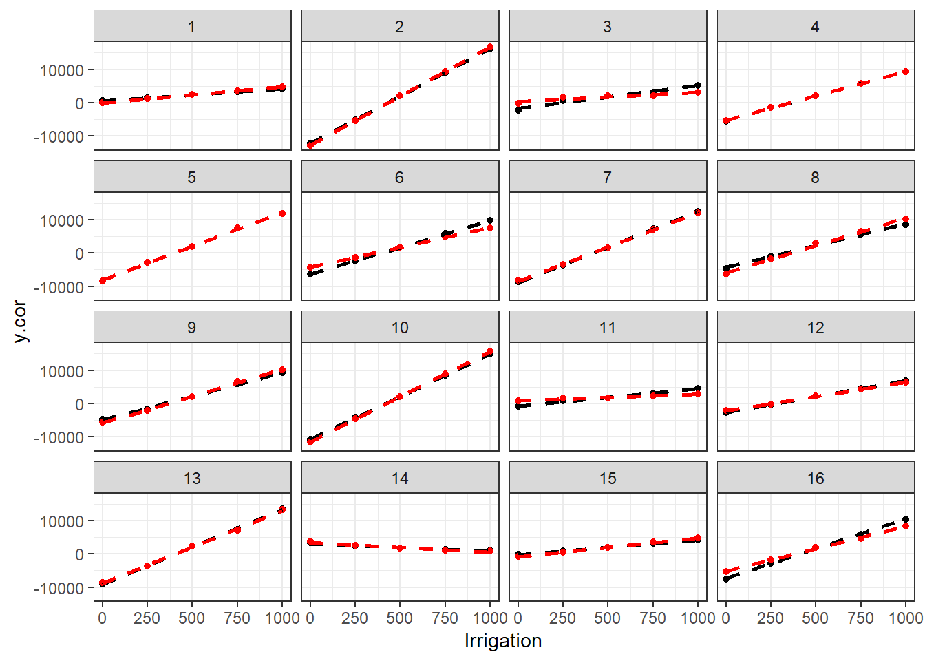
We can see that the new data is very similar to the previous one. The correlation between the random intercepts and slopes is not very strong. But it is sufficient to see that lower intercepts will lead to higher slopes though.
- We can fit both types models to the new dataset:
lmm1a<-lmer(y.cor~ Irrigation.ct + (Irrigation.ct || location),data = design)Warning in checkConv(attr(opt, "derivs"), opt$par, ctrl = control$checkConv, :
Model failed to converge with max|grad| = 0.351015 (tol = 0.002, component 1)lmm1b<-lmer(y.cor~ Irrigation.ct + (Irrigation.ct | location), data = design)Warning in checkConv(attr(opt, "derivs"), opt$par, ctrl = control$checkConv, :
Model failed to converge with max|grad| = 0.0475714 (tol = 0.002, component 1)summary(lmm1a)Linear mixed model fit by REML. t-tests use Satterthwaite's method [
lmerModLmerTest]
Formula: y.cor ~ Irrigation.ct + (Irrigation.ct || location)
Data: design
REML criterion at convergence: 1229.6
Scaled residuals:
Min 1Q Median 3Q Max
-2.17340 -0.56478 -0.01484 0.52740 2.59095
Random effects:
Groups Name Variance Std.Dev.
location (Intercept) 23034.25 151.770
location.1 Irrigation.ct 75.72 8.702
Residual 77040.90 277.562
Number of obs: 80, groups: location, 16
Fixed effects:
Estimate Std. Error df t value Pr(>|t|)
(Intercept) 1973.119 49.017 16.574 40.254 < 2e-16 ***
Irrigation.ct 13.878 2.177 14.984 6.374 1.26e-05 ***
---
Signif. codes: 0 '***' 0.001 '**' 0.01 '*' 0.05 '.' 0.1 ' ' 1
Correlation of Fixed Effects:
(Intr)
Irrigatn.ct 0.000
optimizer (nloptwrap) convergence code: 0 (OK)
Model failed to converge with max|grad| = 0.351015 (tol = 0.002, component 1)summary(lmm1b)Linear mixed model fit by REML. t-tests use Satterthwaite's method [
lmerModLmerTest]
Formula: y.cor ~ Irrigation.ct + (Irrigation.ct | location)
Data: design
REML criterion at convergence: 1229.3
Scaled residuals:
Min 1Q Median 3Q Max
-2.19025 -0.58978 0.01236 0.48375 2.58308
Random effects:
Groups Name Variance Std.Dev. Corr
location (Intercept) 27403.94 165.5
Irrigation.ct 75.68 8.7 -0.15
Residual 74644.40 273.2
Number of obs: 80, groups: location, 16
Fixed effects:
Estimate Std. Error df t value Pr(>|t|)
(Intercept) 1973.119 51.437 14.816 38.360 3.05e-16 ***
Irrigation.ct 13.878 2.177 14.997 6.376 1.25e-05 ***
---
Signif. codes: 0 '***' 0.001 '**' 0.01 '*' 0.05 '.' 0.1 ' ' 1
Correlation of Fixed Effects:
(Intr)
Irrigatn.ct -0.117
optimizer (nloptwrap) convergence code: 0 (OK)
Model failed to converge with max|grad| = 0.0475714 (tol = 0.002, component 1)The estimates of the fixed effects are practically the same. Note that the model does detect a small correlation of about -0.12, which is smaller than the true correlation value we assumed in the data generation.
- We can generate the profile plot for the correlated model:
pr01 <- profile(lmm1b)Warning in nextpar(mat, cc, i, delta, lowcut, upcut): unexpected decrease in
profile: using minstep
Warning in nextpar(mat, cc, i, delta, lowcut, upcut): unexpected decrease in
profile: using minstep
Warning in nextpar(mat, cc, i, delta, lowcut, upcut): unexpected decrease in
profile: using minstepWarning in nextpar(mat, cc, i, delta, lowcut, upcut): Last two rows have
identical or NA .zeta values: using minstep
Warning in nextpar(mat, cc, i, delta, lowcut, upcut): Last two rows have
identical or NA .zeta values: using minstep
Warning in nextpar(mat, cc, i, delta, lowcut, upcut): Last two rows have
identical or NA .zeta values: using minstep
Warning in nextpar(mat, cc, i, delta, lowcut, upcut): Last two rows have
identical or NA .zeta values: using minstep
Warning in nextpar(mat, cc, i, delta, lowcut, upcut): Last two rows have
identical or NA .zeta values: using minstep
Warning in nextpar(mat, cc, i, delta, lowcut, upcut): Last two rows have
identical or NA .zeta values: using minstep
Warning in nextpar(mat, cc, i, delta, lowcut, upcut): Last two rows have
identical or NA .zeta values: using minstep
Warning in nextpar(mat, cc, i, delta, lowcut, upcut): Last two rows have
identical or NA .zeta values: using minstep
Warning in nextpar(mat, cc, i, delta, lowcut, upcut): Last two rows have
identical or NA .zeta values: using minstep
Warning in nextpar(mat, cc, i, delta, lowcut, upcut): Last two rows have
identical or NA .zeta values: using minstep
Warning in nextpar(mat, cc, i, delta, lowcut, upcut): Last two rows have
identical or NA .zeta values: using minstep
Warning in nextpar(mat, cc, i, delta, lowcut, upcut): Last two rows have
identical or NA .zeta values: using minstep
Warning in nextpar(mat, cc, i, delta, lowcut, upcut): Last two rows have
identical or NA .zeta values: using minstep
Warning in nextpar(mat, cc, i, delta, lowcut, upcut): Last two rows have
identical or NA .zeta values: using minstep
Warning in nextpar(mat, cc, i, delta, lowcut, upcut): Last two rows have
identical or NA .zeta values: using minstep
Warning in nextpar(mat, cc, i, delta, lowcut, upcut): Last two rows have
identical or NA .zeta values: using minstep
Warning in nextpar(mat, cc, i, delta, lowcut, upcut): Last two rows have
identical or NA .zeta values: using minstep
Warning in nextpar(mat, cc, i, delta, lowcut, upcut): Last two rows have
identical or NA .zeta values: using minstep
Warning in nextpar(mat, cc, i, delta, lowcut, upcut): Last two rows have
identical or NA .zeta values: using minstep
Warning in nextpar(mat, cc, i, delta, lowcut, upcut): Last two rows have
identical or NA .zeta values: using minstep
Warning in nextpar(mat, cc, i, delta, lowcut, upcut): Last two rows have
identical or NA .zeta values: using minstep
Warning in nextpar(mat, cc, i, delta, lowcut, upcut): Last two rows have
identical or NA .zeta values: using minstep
Warning in nextpar(mat, cc, i, delta, lowcut, upcut): Last two rows have
identical or NA .zeta values: using minstep
Warning in nextpar(mat, cc, i, delta, lowcut, upcut): Last two rows have
identical or NA .zeta values: using minstep
Warning in nextpar(mat, cc, i, delta, lowcut, upcut): Last two rows have
identical or NA .zeta values: using minstep
Warning in nextpar(mat, cc, i, delta, lowcut, upcut): Last two rows have
identical or NA .zeta values: using minstep
Warning in nextpar(mat, cc, i, delta, lowcut, upcut): Last two rows have
identical or NA .zeta values: using minstep
Warning in nextpar(mat, cc, i, delta, lowcut, upcut): Last two rows have
identical or NA .zeta values: using minstep
Warning in nextpar(mat, cc, i, delta, lowcut, upcut): Last two rows have
identical or NA .zeta values: using minstep
Warning in nextpar(mat, cc, i, delta, lowcut, upcut): Last two rows have
identical or NA .zeta values: using minstep
Warning in nextpar(mat, cc, i, delta, lowcut, upcut): Last two rows have
identical or NA .zeta values: using minstep
Warning in nextpar(mat, cc, i, delta, lowcut, upcut): Last two rows have
identical or NA .zeta values: using minstep
Warning in nextpar(mat, cc, i, delta, lowcut, upcut): Last two rows have
identical or NA .zeta values: using minstep
Warning in nextpar(mat, cc, i, delta, lowcut, upcut): Last two rows have
identical or NA .zeta values: using minstep
Warning in nextpar(mat, cc, i, delta, lowcut, upcut): Last two rows have
identical or NA .zeta values: using minstep
Warning in nextpar(mat, cc, i, delta, lowcut, upcut): Last two rows have
identical or NA .zeta values: using minstep
Warning in nextpar(mat, cc, i, delta, lowcut, upcut): Last two rows have
identical or NA .zeta values: using minstep
Warning in nextpar(mat, cc, i, delta, lowcut, upcut): Last two rows have
identical or NA .zeta values: using minstep
Warning in nextpar(mat, cc, i, delta, lowcut, upcut): Last two rows have
identical or NA .zeta values: using minstep
Warning in nextpar(mat, cc, i, delta, lowcut, upcut): Last two rows have
identical or NA .zeta values: using minstep
Warning in nextpar(mat, cc, i, delta, lowcut, upcut): Last two rows have
identical or NA .zeta values: using minstep
Warning in nextpar(mat, cc, i, delta, lowcut, upcut): Last two rows have
identical or NA .zeta values: using minstep
Warning in nextpar(mat, cc, i, delta, lowcut, upcut): Last two rows have
identical or NA .zeta values: using minstep
Warning in nextpar(mat, cc, i, delta, lowcut, upcut): Last two rows have
identical or NA .zeta values: using minstep
Warning in nextpar(mat, cc, i, delta, lowcut, upcut): Last two rows have
identical or NA .zeta values: using minstep
Warning in nextpar(mat, cc, i, delta, lowcut, upcut): Last two rows have
identical or NA .zeta values: using minstep
Warning in nextpar(mat, cc, i, delta, lowcut, upcut): Last two rows have
identical or NA .zeta values: using minstep
Warning in nextpar(mat, cc, i, delta, lowcut, upcut): Last two rows have
identical or NA .zeta values: using minstep
Warning in nextpar(mat, cc, i, delta, lowcut, upcut): Last two rows have
identical or NA .zeta values: using minstep
Warning in nextpar(mat, cc, i, delta, lowcut, upcut): Last two rows have
identical or NA .zeta values: using minstep
Warning in nextpar(mat, cc, i, delta, lowcut, upcut): Last two rows have
identical or NA .zeta values: using minstep
Warning in nextpar(mat, cc, i, delta, lowcut, upcut): Last two rows have
identical or NA .zeta values: using minstep
Warning in nextpar(mat, cc, i, delta, lowcut, upcut): Last two rows have
identical or NA .zeta values: using minstep
Warning in nextpar(mat, cc, i, delta, lowcut, upcut): Last two rows have
identical or NA .zeta values: using minstep
Warning in nextpar(mat, cc, i, delta, lowcut, upcut): Last two rows have
identical or NA .zeta values: using minstep
Warning in nextpar(mat, cc, i, delta, lowcut, upcut): Last two rows have
identical or NA .zeta values: using minstep
Warning in nextpar(mat, cc, i, delta, lowcut, upcut): Last two rows have
identical or NA .zeta values: using minstep
Warning in nextpar(mat, cc, i, delta, lowcut, upcut): Last two rows have
identical or NA .zeta values: using minstep
Warning in nextpar(mat, cc, i, delta, lowcut, upcut): Last two rows have
identical or NA .zeta values: using minstep
Warning in nextpar(mat, cc, i, delta, lowcut, upcut): Last two rows have
identical or NA .zeta values: using minstep
Warning in nextpar(mat, cc, i, delta, lowcut, upcut): Last two rows have
identical or NA .zeta values: using minstep
Warning in nextpar(mat, cc, i, delta, lowcut, upcut): Last two rows have
identical or NA .zeta values: using minstep
Warning in nextpar(mat, cc, i, delta, lowcut, upcut): Last two rows have
identical or NA .zeta values: using minstep
Warning in nextpar(mat, cc, i, delta, lowcut, upcut): Last two rows have
identical or NA .zeta values: using minstep
Warning in nextpar(mat, cc, i, delta, lowcut, upcut): Last two rows have
identical or NA .zeta values: using minstep
Warning in nextpar(mat, cc, i, delta, lowcut, upcut): Last two rows have
identical or NA .zeta values: using minstep
Warning in nextpar(mat, cc, i, delta, lowcut, upcut): Last two rows have
identical or NA .zeta values: using minstep
Warning in nextpar(mat, cc, i, delta, lowcut, upcut): Last two rows have
identical or NA .zeta values: using minstep
Warning in nextpar(mat, cc, i, delta, lowcut, upcut): Last two rows have
identical or NA .zeta values: using minstep
Warning in nextpar(mat, cc, i, delta, lowcut, upcut): Last two rows have
identical or NA .zeta values: using minstep
Warning in nextpar(mat, cc, i, delta, lowcut, upcut): Last two rows have
identical or NA .zeta values: using minstep
Warning in nextpar(mat, cc, i, delta, lowcut, upcut): Last two rows have
identical or NA .zeta values: using minstep
Warning in nextpar(mat, cc, i, delta, lowcut, upcut): Last two rows have
identical or NA .zeta values: using minstep
Warning in nextpar(mat, cc, i, delta, lowcut, upcut): Last two rows have
identical or NA .zeta values: using minstep
Warning in nextpar(mat, cc, i, delta, lowcut, upcut): Last two rows have
identical or NA .zeta values: using minstep
Warning in nextpar(mat, cc, i, delta, lowcut, upcut): Last two rows have
identical or NA .zeta values: using minstep
Warning in nextpar(mat, cc, i, delta, lowcut, upcut): Last two rows have
identical or NA .zeta values: using minstep
Warning in nextpar(mat, cc, i, delta, lowcut, upcut): Last two rows have
identical or NA .zeta values: using minstep
Warning in nextpar(mat, cc, i, delta, lowcut, upcut): Last two rows have
identical or NA .zeta values: using minstep
Warning in nextpar(mat, cc, i, delta, lowcut, upcut): Last two rows have
identical or NA .zeta values: using minstep
Warning in nextpar(mat, cc, i, delta, lowcut, upcut): Last two rows have
identical or NA .zeta values: using minstep
Warning in nextpar(mat, cc, i, delta, lowcut, upcut): Last two rows have
identical or NA .zeta values: using minstep
Warning in nextpar(mat, cc, i, delta, lowcut, upcut): Last two rows have
identical or NA .zeta values: using minstep
Warning in nextpar(mat, cc, i, delta, lowcut, upcut): Last two rows have
identical or NA .zeta values: using minstep
Warning in nextpar(mat, cc, i, delta, lowcut, upcut): Last two rows have
identical or NA .zeta values: using minstep
Warning in nextpar(mat, cc, i, delta, lowcut, upcut): Last two rows have
identical or NA .zeta values: using minstep
Warning in nextpar(mat, cc, i, delta, lowcut, upcut): Last two rows have
identical or NA .zeta values: using minstep
Warning in nextpar(mat, cc, i, delta, lowcut, upcut): Last two rows have
identical or NA .zeta values: using minstepWarning in FUN(X[[i]], ...): non-monotonic profile for .sig02xyplot(pr01, aspect = 1.3)Warning in regularize.values(x, y, ties, missing(ties), na.rm = na.rm):
collapsing to unique 'x' valuesWarning in (function (x, y, spl, absVal, ...) : bad profile for variable 2:
using linear interpolation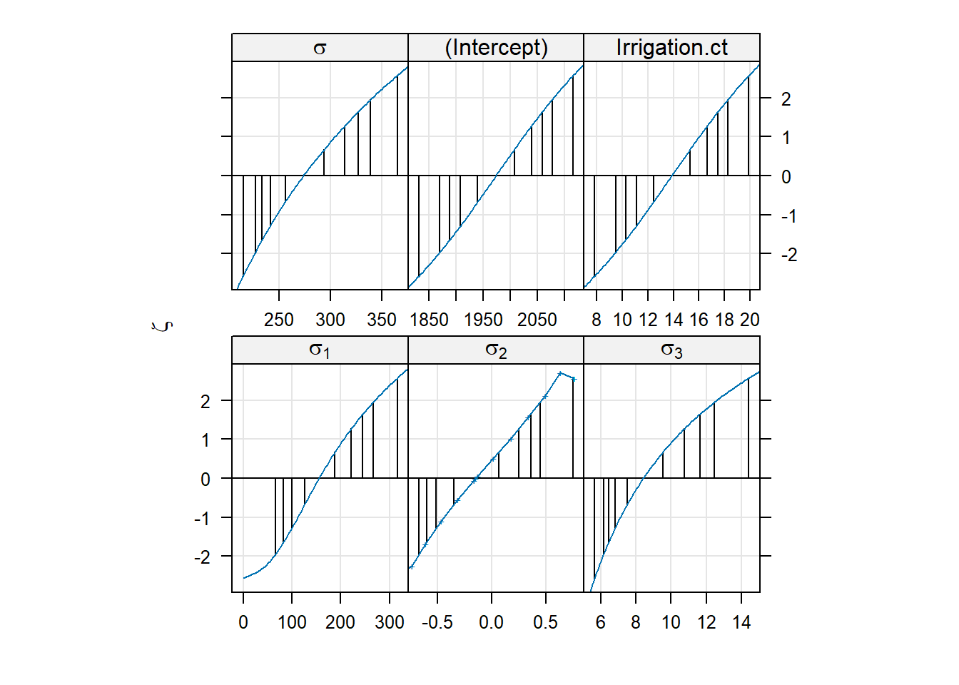
We get a series of warnings that R is struggling to calculate some of the profiles, and we can see a bad profile with one of the variance components. This is a sign that the model is not well identified and that the profiles may not be reliable.
We know that the model with correlation is better than the one without, because we know the true underlying process that generated the data. In the real world this information is not available and we cannot assume that we have the “true” model (in fact, one critique of this kind of simulation studies is that assumes we know the model that generated the data and only have to estimate the parameters). Therefore, we need to use other criteria to decide which model is better. When we are doubting whether to include a fixed effect or not, the F test that we have discussed in previous chapters is a good criterion. However, there are no F tests for random effects. Instead, we can use the likelihood ratio test:
anova(lmm1a, lmm1b)refitting model(s) with ML (instead of REML)Data: design
Models:
lmm1a: y.cor ~ Irrigation.ct + (Irrigation.ct || location)
lmm1b: y.cor ~ Irrigation.ct + (Irrigation.ct | location)
npar AIC BIC logLik -2*log(L) Chisq Df Pr(>Chisq)
lmm1a 5 1252.5 1264.4 -621.26 1242.5
lmm1b 6 1254.3 1268.6 -621.15 1242.3 0.2222 1 0.6374We can see that the likelihood ratio test is not significant, which means that the model with correlation is not considered to be better than the one without correlation (despite the fact that we know it is closer to the true model). This is a consequenc of (i) sampling error and (ii) the fact that the fitting algorithm did not fully converged and the model was not fully estimated (see the warning messages above).The latter is an error will start to show up more often as we increase the complexity of the model. Later in the course we will learn the Bayesian paradigm of parameter estimation that can address these convergence issues better.
From this comparison we would conclude that there is no sufficient evidence for correlation between random intercepts and slopes and therefore the simpler model is preferred (see Occams’ razor).
6.4 A more complex example: Effect of P nutrition on yield across farms
Read in the data:
pke.dat <- read.csv("data/raw/nigeria.pke.dat.csv")Create new variables to encode P fertilization treatment vs control (ignoring the other nutrients). First we create the special label encoding each treatment with a 0 or 1:
pke.dat$treat <- with(pke.dat,paste(i,p,k,e,om, sep = ""))Then we create a new variable that encodes the treatment as a factor and we order the data according to the different relevant factors:
pke.dat$treat.p <- NA
pke.dat$treat.p[pke.dat$treat=="00000"|pke.dat$treat=="10000"] <- "control"
pke.dat$treat.p[pke.dat$treat=="11000"|pke.dat$treat=="11100"|
                pke.dat$treat=="11110"|pke.dat$treat=="11111"] <- "+p"
indices <- with(pke.dat, order(district, year, farm_id, treat.p))
pke.dat <- pke.dat[indices,]
We also need to create a dummy variable to encode the random slopes:
pke.dat$x1 <- ifelse(pke.dat$treat.p == "control", 0, 1)Exercise 6.3
- Fit two linear mixed models with random intercepts and slopes, one where these are correlated and one where they are not. Use
k,e,omandx1as fixed effects. and consider the following nested structure:district/year/farm_id. - Compare the models using the likelihood ratio test, which one is best?
- Continue with the best model and check the reliability of the parameter estimates using the profile plot.
- Check whether the assumption of normality and homoscedasticity of the residuals is met.
Solution 6.3
- We can fit the models as follows:
# with correlation
lmm1a <- lmer(estimated.grain.yield_kg_ha~k + e + om + x1 + (1 + x1| district / year /
              farm_id), data= pke.dat)
# without correlation
lmm1b <- lmer(estimated.grain.yield_kg_ha~k + e + om + x1 + (1 + x1 || district / year /
farm_id), data= pke.dat)- We can compare the models using the likelihood ratio test:
anova(lmm1a, lmm1b)refitting model(s) with ML (instead of REML)Data: pke.dat
Models:
lmm1b: estimated.grain.yield_kg_ha ~ k + e + om + x1 + (1 + x1 || district/year/farm_id)
lmm1a: estimated.grain.yield_kg_ha ~ k + e + om + x1 + (1 + x1 | district/year/farm_id)
npar AIC BIC logLik -2*log(L) Chisq Df Pr(>Chisq)
lmm1b 12 11548 11604 -5762.2 11524
lmm1a 15 11551 11621 -5760.5 11521 3.5414 3 0.3154The best model is the one without correlation as adding correlation does not improve the likelihood well enough to justify the extra complexity.
- We can check the reliability of the parameter estimates using the profile plot:
pr01 <- profile(lmm1b)Warning in nextpar(mat, cc, i, delta, lowcut, upcut): Last two rows have
identical or NA .zeta values: using minstep
Warning in nextpar(mat, cc, i, delta, lowcut, upcut): Last two rows have
identical or NA .zeta values: using minstep
Warning in nextpar(mat, cc, i, delta, lowcut, upcut): Last two rows have
identical or NA .zeta values: using minstep
Warning in nextpar(mat, cc, i, delta, lowcut, upcut): Last two rows have
identical or NA .zeta values: using minstep
Warning in nextpar(mat, cc, i, delta, lowcut, upcut): Last two rows have
identical or NA .zeta values: using minstep
Warning in nextpar(mat, cc, i, delta, lowcut, upcut): Last two rows have
identical or NA .zeta values: using minstep
Warning in nextpar(mat, cc, i, delta, lowcut, upcut): Last two rows have
identical or NA .zeta values: using minstep
Warning in nextpar(mat, cc, i, delta, lowcut, upcut): Last two rows have
identical or NA .zeta values: using minstepWarning in nextpar(mat, cc, i, delta, lowcut, upcut): unexpected decrease in
profile: using minstepWarning in nextpar(mat, cc, i, delta, lowcut, upcut): Last two rows have
identical or NA .zeta values: using minstep
Warning in nextpar(mat, cc, i, delta, lowcut, upcut): Last two rows have
identical or NA .zeta values: using minstep
Warning in nextpar(mat, cc, i, delta, lowcut, upcut): Last two rows have
identical or NA .zeta values: using minstep
Warning in nextpar(mat, cc, i, delta, lowcut, upcut): Last two rows have
identical or NA .zeta values: using minstep
Warning in nextpar(mat, cc, i, delta, lowcut, upcut): Last two rows have
identical or NA .zeta values: using minstep
Warning in nextpar(mat, cc, i, delta, lowcut, upcut): Last two rows have
identical or NA .zeta values: using minstep
Warning in nextpar(mat, cc, i, delta, lowcut, upcut): Last two rows have
identical or NA .zeta values: using minstepWarning in nextpar(mat, cc, i, delta, lowcut, upcut): unexpected decrease in
profile: using minstepWarning in nextpar(mat, cc, i, delta, lowcut, upcut): Last two rows have
identical or NA .zeta values: using minstepWarning in nextpar(mat, cc, i, delta, lowcut, upcut): unexpected decrease in
profile: using minstepWarning in nextpar(mat, cc, i, delta, lowcut, upcut): Last two rows have
identical or NA .zeta values: using minstep
Warning in nextpar(mat, cc, i, delta, lowcut, upcut): Last two rows have
identical or NA .zeta values: using minstep
Warning in nextpar(mat, cc, i, delta, lowcut, upcut): Last two rows have
identical or NA .zeta values: using minstep
Warning in nextpar(mat, cc, i, delta, lowcut, upcut): Last two rows have
identical or NA .zeta values: using minstep
Warning in nextpar(mat, cc, i, delta, lowcut, upcut): Last two rows have
identical or NA .zeta values: using minstep
Warning in nextpar(mat, cc, i, delta, lowcut, upcut): Last two rows have
identical or NA .zeta values: using minstep
Warning in nextpar(mat, cc, i, delta, lowcut, upcut): Last two rows have
identical or NA .zeta values: using minstep
Warning in nextpar(mat, cc, i, delta, lowcut, upcut): Last two rows have
identical or NA .zeta values: using minstep
Warning in nextpar(mat, cc, i, delta, lowcut, upcut): Last two rows have
identical or NA .zeta values: using minstep
Warning in nextpar(mat, cc, i, delta, lowcut, upcut): Last two rows have
identical or NA .zeta values: using minstep
Warning in nextpar(mat, cc, i, delta, lowcut, upcut): Last two rows have
identical or NA .zeta values: using minstep
Warning in nextpar(mat, cc, i, delta, lowcut, upcut): Last two rows have
identical or NA .zeta values: using minstep
Warning in nextpar(mat, cc, i, delta, lowcut, upcut): Last two rows have
identical or NA .zeta values: using minstep
Warning in nextpar(mat, cc, i, delta, lowcut, upcut): Last two rows have
identical or NA .zeta values: using minstep
Warning in nextpar(mat, cc, i, delta, lowcut, upcut): Last two rows have
identical or NA .zeta values: using minstep
Warning in nextpar(mat, cc, i, delta, lowcut, upcut): Last two rows have
identical or NA .zeta values: using minstep
Warning in nextpar(mat, cc, i, delta, lowcut, upcut): Last two rows have
identical or NA .zeta values: using minstep
Warning in nextpar(mat, cc, i, delta, lowcut, upcut): Last two rows have
identical or NA .zeta values: using minstep
Warning in nextpar(mat, cc, i, delta, lowcut, upcut): Last two rows have
identical or NA .zeta values: using minstep
Warning in nextpar(mat, cc, i, delta, lowcut, upcut): Last two rows have
identical or NA .zeta values: using minstep
Warning in nextpar(mat, cc, i, delta, lowcut, upcut): Last two rows have
identical or NA .zeta values: using minstep
Warning in nextpar(mat, cc, i, delta, lowcut, upcut): Last two rows have
identical or NA .zeta values: using minstep
Warning in nextpar(mat, cc, i, delta, lowcut, upcut): Last two rows have
identical or NA .zeta values: using minstep
Warning in nextpar(mat, cc, i, delta, lowcut, upcut): Last two rows have
identical or NA .zeta values: using minstep
Warning in nextpar(mat, cc, i, delta, lowcut, upcut): Last two rows have
identical or NA .zeta values: using minstep
Warning in nextpar(mat, cc, i, delta, lowcut, upcut): Last two rows have
identical or NA .zeta values: using minstep
Warning in nextpar(mat, cc, i, delta, lowcut, upcut): Last two rows have
identical or NA .zeta values: using minstep
Warning in nextpar(mat, cc, i, delta, lowcut, upcut): Last two rows have
identical or NA .zeta values: using minstep
Warning in nextpar(mat, cc, i, delta, lowcut, upcut): Last two rows have
identical or NA .zeta values: using minstep
Warning in nextpar(mat, cc, i, delta, lowcut, upcut): Last two rows have
identical or NA .zeta values: using minstep
Warning in nextpar(mat, cc, i, delta, lowcut, upcut): Last two rows have
identical or NA .zeta values: using minstep
Warning in nextpar(mat, cc, i, delta, lowcut, upcut): Last two rows have
identical or NA .zeta values: using minstep
Warning in nextpar(mat, cc, i, delta, lowcut, upcut): Last two rows have
identical or NA .zeta values: using minstep
Warning in nextpar(mat, cc, i, delta, lowcut, upcut): Last two rows have
identical or NA .zeta values: using minstep
Warning in nextpar(mat, cc, i, delta, lowcut, upcut): Last two rows have
identical or NA .zeta values: using minstep
Warning in nextpar(mat, cc, i, delta, lowcut, upcut): Last two rows have
identical or NA .zeta values: using minstep
Warning in nextpar(mat, cc, i, delta, lowcut, upcut): Last two rows have
identical or NA .zeta values: using minstep
Warning in nextpar(mat, cc, i, delta, lowcut, upcut): Last two rows have
identical or NA .zeta values: using minstep
Warning in nextpar(mat, cc, i, delta, lowcut, upcut): Last two rows have
identical or NA .zeta values: using minstep
Warning in nextpar(mat, cc, i, delta, lowcut, upcut): Last two rows have
identical or NA .zeta values: using minstep
Warning in nextpar(mat, cc, i, delta, lowcut, upcut): Last two rows have
identical or NA .zeta values: using minstep
Warning in nextpar(mat, cc, i, delta, lowcut, upcut): Last two rows have
identical or NA .zeta values: using minstep
Warning in nextpar(mat, cc, i, delta, lowcut, upcut): Last two rows have
identical or NA .zeta values: using minstepWarning in nextpar(mat, cc, i, delta, lowcut, upcut): unexpected decrease in
profile: using minstepWarning in nextpar(mat, cc, i, delta, lowcut, upcut): Last two rows have
identical or NA .zeta values: using minstep
Warning in nextpar(mat, cc, i, delta, lowcut, upcut): Last two rows have
identical or NA .zeta values: using minstep
Warning in nextpar(mat, cc, i, delta, lowcut, upcut): Last two rows have
identical or NA .zeta values: using minstep
Warning in nextpar(mat, cc, i, delta, lowcut, upcut): Last two rows have
identical or NA .zeta values: using minstep
Warning in nextpar(mat, cc, i, delta, lowcut, upcut): Last two rows have
identical or NA .zeta values: using minstep
Warning in nextpar(mat, cc, i, delta, lowcut, upcut): Last two rows have
identical or NA .zeta values: using minstep
Warning in nextpar(mat, cc, i, delta, lowcut, upcut): Last two rows have
identical or NA .zeta values: using minstep
Warning in nextpar(mat, cc, i, delta, lowcut, upcut): Last two rows have
identical or NA .zeta values: using minstep
Warning in nextpar(mat, cc, i, delta, lowcut, upcut): Last two rows have
identical or NA .zeta values: using minstepWarning in nextpar(mat, cc, i, delta, lowcut, upcut): unexpected decrease in
profile: using minstepWarning in nextpar(mat, cc, i, delta, lowcut, upcut): Last two rows have
identical or NA .zeta values: using minstep
Warning in nextpar(mat, cc, i, delta, lowcut, upcut): Last two rows have
identical or NA .zeta values: using minstep
Warning in nextpar(mat, cc, i, delta, lowcut, upcut): Last two rows have
identical or NA .zeta values: using minstepWarning in nextpar(mat, cc, i, delta, lowcut, upcut): unexpected decrease in
profile: using minstepWarning in nextpar(mat, cc, i, delta, lowcut, upcut): Last two rows have
identical or NA .zeta values: using minstepWarning in nextpar(mat, cc, i, delta, lowcut, upcut): unexpected decrease in
profile: using minstep
Warning in nextpar(mat, cc, i, delta, lowcut, upcut): unexpected decrease in
profile: using minstep
Warning in nextpar(mat, cc, i, delta, lowcut, upcut): Last two rows have
identical or NA .zeta values: using minstep
Warning in nextpar(mat, cc, i, delta, lowcut, upcut): Last two rows have
identical or NA .zeta values: using minstep
Warning in nextpar(mat, cc, i, delta, lowcut, upcut): Last two rows have
identical or NA .zeta values: using minstep
Warning in zetafun(np, ns): slightly lower deviances (diff=-1.81899e-12)
detectedWarning in nextpar(mat, cc, i, delta, lowcut, upcut): Last two rows have
identical or NA .zeta values: using minstepWarning in zetafun(np, ns): slightly lower deviances (diff=-1.81899e-12)
detectedWarning in nextpar(mat, cc, i, delta, lowcut, upcut): Last two rows have
identical or NA .zeta values: using minstepWarning in zetafun(np, ns): slightly lower deviances (diff=-1.81899e-12)
detectedWarning in nextpar(mat, cc, i, delta, lowcut, upcut): Last two rows have
identical or NA .zeta values: using minstepWarning in zetafun(np, ns): slightly lower deviances (diff=-1.81899e-12)
detectedWarning in nextpar(mat, cc, i, delta, lowcut, upcut): Last two rows have
identical or NA .zeta values: using minstepWarning in zetafun(np, ns): slightly lower deviances (diff=-1.81899e-12)
detectedWarning in nextpar(mat, cc, i, delta, lowcut, upcut): Last two rows have
identical or NA .zeta values: using minstepWarning in zetafun(np, ns): slightly lower deviances (diff=-1.81899e-12)
detectedWarning in nextpar(mat, cc, i, delta, lowcut, upcut): Last two rows have
identical or NA .zeta values: using minstep
Warning in nextpar(mat, cc, i, delta, lowcut, upcut): Last two rows have
identical or NA .zeta values: using minstep
Warning in zetafun(np, ns): slightly lower deviances (diff=-1.81899e-12)
detectedWarning in nextpar(mat, cc, i, delta, lowcut, upcut): Last two rows have
identical or NA .zeta values: using minstepWarning in zetafun(np, ns): slightly lower deviances (diff=-1.81899e-12)
detectedWarning in nextpar(mat, cc, i, delta, lowcut, upcut): Last two rows have
identical or NA .zeta values: using minstepWarning in zetafun(np, ns): slightly lower deviances (diff=-1.81899e-12)
detectedWarning in nextpar(mat, cc, i, delta, lowcut, upcut): Last two rows have
identical or NA .zeta values: using minstepWarning in zetafun(np, ns): slightly lower deviances (diff=-1.81899e-12)
detectedWarning in nextpar(mat, cc, i, delta, lowcut, upcut): Last two rows have
identical or NA .zeta values: using minstepWarning in zetafun(np, ns): slightly lower deviances (diff=-1.81899e-12)
detectedWarning in nextpar(mat, cc, i, delta, lowcut, upcut): Last two rows have
identical or NA .zeta values: using minstepWarning in zetafun(np, ns): slightly lower deviances (diff=-1.81899e-12)
detectedWarning in nextpar(mat, cc, i, delta, lowcut, upcut): Last two rows have
identical or NA .zeta values: using minstepWarning in zetafun(np, ns): slightly lower deviances (diff=-1.81899e-12)
detectedWarning in nextpar(mat, cc, i, delta, lowcut, upcut): Last two rows have
identical or NA .zeta values: using minstepWarning in zetafun(np, ns): slightly lower deviances (diff=-1.81899e-12)
detectedWarning in nextpar(mat, cc, i, delta, lowcut, upcut): Last two rows have
identical or NA .zeta values: using minstepWarning in zetafun(np, ns): slightly lower deviances (diff=-1.81899e-12)
detectedWarning in nextpar(mat, cc, i, delta, lowcut, upcut): Last two rows have
identical or NA .zeta values: using minstepWarning in zetafun(np, ns): slightly lower deviances (diff=-1.81899e-12)
detectedWarning in nextpar(mat, cc, i, delta, lowcut, upcut): Last two rows have
identical or NA .zeta values: using minstepWarning in zetafun(np, ns): slightly lower deviances (diff=-1.81899e-12)
detectedWarning in nextpar(mat, cc, i, delta, lowcut, upcut): Last two rows have
identical or NA .zeta values: using minstepWarning in zetafun(np, ns): slightly lower deviances (diff=-1.81899e-12)
detectedWarning in nextpar(mat, cc, i, delta, lowcut, upcut): Last two rows have
identical or NA .zeta values: using minstepWarning in zetafun(np, ns): slightly lower deviances (diff=-1.81899e-12)
detectedWarning in nextpar(mat, cc, i, delta, lowcut, upcut): Last two rows have
identical or NA .zeta values: using minstepWarning in zetafun(np, ns): slightly lower deviances (diff=-1.81899e-12)
detectedWarning in nextpar(mat, cc, i, delta, lowcut, upcut): Last two rows have
identical or NA .zeta values: using minstepWarning in zetafun(np, ns): slightly lower deviances (diff=-1.81899e-12)
detectedWarning in nextpar(mat, cc, i, delta, lowcut, upcut): Last two rows have
identical or NA .zeta values: using minstepWarning in zetafun(np, ns): slightly lower deviances (diff=-1.81899e-12)
detectedWarning in nextpar(mat, cc, i, delta, lowcut, upcut): Last two rows have
identical or NA .zeta values: using minstepWarning in zetafun(np, ns): slightly lower deviances (diff=-1.81899e-12)
detectedWarning in nextpar(mat, cc, i, delta, lowcut, upcut): Last two rows have
identical or NA .zeta values: using minstepWarning in zetafun(np, ns): slightly lower deviances (diff=-1.81899e-12)
detectedWarning in nextpar(mat, cc, i, delta, lowcut, upcut): Last two rows have
identical or NA .zeta values: using minstepWarning in zetafun(np, ns): slightly lower deviances (diff=-1.81899e-12)
detectedWarning in nextpar(mat, cc, i, delta, lowcut, upcut): Last two rows have
identical or NA .zeta values: using minstepWarning in zetafun(np, ns): slightly lower deviances (diff=-1.81899e-12)
detectedWarning in nextpar(mat, cc, i, delta, lowcut, upcut): Last two rows have
identical or NA .zeta values: using minstepWarning in zetafun(np, ns): slightly lower deviances (diff=-1.81899e-12)
detectedWarning in nextpar(mat, cc, i, delta, lowcut, upcut): Last two rows have
identical or NA .zeta values: using minstepWarning in zetafun(np, ns): slightly lower deviances (diff=-1.81899e-12)
detectedWarning in nextpar(mat, cc, i, delta, lowcut, upcut): Last two rows have
identical or NA .zeta values: using minstepWarning in zetafun(np, ns): slightly lower deviances (diff=-1.81899e-12)
detectedWarning in nextpar(mat, cc, i, delta, lowcut, upcut): Last two rows have
identical or NA .zeta values: using minstepWarning in zetafun(np, ns): slightly lower deviances (diff=-1.81899e-12)
detectedWarning in nextpar(mat, cc, i, delta, lowcut, upcut): Last two rows have
identical or NA .zeta values: using minstepWarning in zetafun(np, ns): slightly lower deviances (diff=-1.81899e-12)
detectedWarning in nextpar(mat, cc, i, delta, lowcut, upcut): Last two rows have
identical or NA .zeta values: using minstepWarning in zetafun(np, ns): slightly lower deviances (diff=-1.81899e-12)
detectedWarning in nextpar(mat, cc, i, delta, lowcut, upcut): Last two rows have
identical or NA .zeta values: using minstepWarning in zetafun(np, ns): slightly lower deviances (diff=-1.81899e-12)
detectedWarning in nextpar(mat, cc, i, delta, lowcut, upcut): Last two rows have
identical or NA .zeta values: using minstepWarning in zetafun(np, ns): slightly lower deviances (diff=-1.81899e-12)
detectedWarning in nextpar(mat, cc, i, delta, lowcut, upcut): Last two rows have
identical or NA .zeta values: using minstepWarning in zetafun(np, ns): slightly lower deviances (diff=-1.81899e-12)
detectedWarning in nextpar(mat, cc, i, delta, lowcut, upcut): Last two rows have
identical or NA .zeta values: using minstepWarning in zetafun(np, ns): slightly lower deviances (diff=-1.81899e-12)
detectedWarning in nextpar(mat, cc, i, delta, lowcut, upcut): Last two rows have
identical or NA .zeta values: using minstepWarning in zetafun(np, ns): slightly lower deviances (diff=-1.81899e-12)
detectedWarning in nextpar(mat, cc, i, delta, lowcut, upcut): Last two rows have
identical or NA .zeta values: using minstepWarning in zetafun(np, ns): slightly lower deviances (diff=-1.81899e-12)
detectedWarning in nextpar(mat, cc, i, delta, lowcut, upcut): Last two rows have
identical or NA .zeta values: using minstepWarning in zetafun(np, ns): slightly lower deviances (diff=-1.81899e-12)
detectedWarning in nextpar(mat, cc, i, delta, lowcut, upcut): Last two rows have
identical or NA .zeta values: using minstepWarning in zetafun(np, ns): slightly lower deviances (diff=-1.81899e-12)
detectedWarning in nextpar(mat, cc, i, delta, lowcut, upcut): Last two rows have
identical or NA .zeta values: using minstepWarning in zetafun(np, ns): slightly lower deviances (diff=-1.81899e-12)
detectedWarning in nextpar(mat, cc, i, delta, lowcut, upcut): Last two rows have
identical or NA .zeta values: using minstepWarning in zetafun(np, ns): slightly lower deviances (diff=-1.81899e-12)
detectedWarning in nextpar(mat, cc, i, delta, lowcut, upcut): Last two rows have
identical or NA .zeta values: using minstepWarning in zetafun(np, ns): slightly lower deviances (diff=-1.81899e-12)
detectedWarning in nextpar(mat, cc, i, delta, lowcut, upcut): Last two rows have
identical or NA .zeta values: using minstepWarning in zetafun(np, ns): slightly lower deviances (diff=-1.81899e-12)
detectedWarning in nextpar(mat, cc, i, delta, lowcut, upcut): Last two rows have
identical or NA .zeta values: using minstepWarning in zetafun(np, ns): slightly lower deviances (diff=-1.81899e-12)
detectedWarning in nextpar(mat, cc, i, delta, lowcut, upcut): Last two rows have
identical or NA .zeta values: using minstepWarning in zetafun(np, ns): slightly lower deviances (diff=-1.81899e-12)
detectedWarning in nextpar(mat, cc, i, delta, lowcut, upcut): Last two rows have
identical or NA .zeta values: using minstepWarning in zetafun(np, ns): slightly lower deviances (diff=-1.81899e-12)
detectedWarning in nextpar(mat, cc, i, delta, lowcut, upcut): Last two rows have
identical or NA .zeta values: using minstepWarning in zetafun(np, ns): slightly lower deviances (diff=-1.81899e-12)
detectedWarning in nextpar(mat, cc, i, delta, lowcut, upcut): Last two rows have
identical or NA .zeta values: using minstepWarning in zetafun(np, ns): slightly lower deviances (diff=-1.81899e-12)
detectedWarning in nextpar(mat, cc, i, delta, lowcut, upcut): Last two rows have
identical or NA .zeta values: using minstepWarning in zetafun(np, ns): slightly lower deviances (diff=-1.81899e-12)
detectedWarning in nextpar(mat, cc, i, delta, lowcut, upcut): Last two rows have
identical or NA .zeta values: using minstepWarning in zetafun(np, ns): slightly lower deviances (diff=-1.81899e-12)
detectedWarning in nextpar(mat, cc, i, delta, lowcut, upcut): Last two rows have
identical or NA .zeta values: using minstepWarning in zetafun(np, ns): slightly lower deviances (diff=-1.81899e-12)
detectedWarning in nextpar(mat, cc, i, delta, lowcut, upcut): Last two rows have
identical or NA .zeta values: using minstepWarning in zetafun(np, ns): slightly lower deviances (diff=-1.81899e-12)
detectedWarning in nextpar(mat, cc, i, delta, lowcut, upcut): Last two rows have
identical or NA .zeta values: using minstepWarning in zetafun(np, ns): slightly lower deviances (diff=-1.81899e-12)
detectedWarning in nextpar(mat, cc, i, delta, lowcut, upcut): Last two rows have
identical or NA .zeta values: using minstepWarning in zetafun(np, ns): slightly lower deviances (diff=-1.81899e-12)
detectedWarning in nextpar(mat, cc, i, delta, lowcut, upcut): Last two rows have
identical or NA .zeta values: using minstepWarning in zetafun(np, ns): slightly lower deviances (diff=-1.81899e-12)
detectedWarning in nextpar(mat, cc, i, delta, lowcut, upcut): Last two rows have
identical or NA .zeta values: using minstep
Warning in nextpar(mat, cc, i, delta, lowcut, upcut): Last two rows have
identical or NA .zeta values: using minstep
Warning in zetafun(np, ns): slightly lower deviances (diff=-1.81899e-12)
detectedWarning in nextpar(mat, cc, i, delta, lowcut, upcut): Last two rows have
identical or NA .zeta values: using minstepWarning in zetafun(np, ns): slightly lower deviances (diff=-1.81899e-12)
detectedWarning in nextpar(mat, cc, i, delta, lowcut, upcut): Last two rows have
identical or NA .zeta values: using minstepWarning in zetafun(np, ns): slightly lower deviances (diff=-1.81899e-12)
detectedWarning in nextpar(mat, cc, i, delta, lowcut, upcut): Last two rows have
identical or NA .zeta values: using minstepWarning in zetafun(np, ns): slightly lower deviances (diff=-1.81899e-12)
detectedWarning in nextpar(mat, cc, i, delta, lowcut, upcut): Last two rows have
identical or NA .zeta values: using minstepWarning in zetafun(np, ns): slightly lower deviances (diff=-1.81899e-12)
detectedWarning in nextpar(mat, cc, i, delta, lowcut, upcut): Last two rows have
identical or NA .zeta values: using minstepWarning in zetafun(np, ns): slightly lower deviances (diff=-1.81899e-12)
detectedWarning in nextpar(mat, cc, i, delta, lowcut, upcut): Last two rows have
identical or NA .zeta values: using minstepWarning in zetafun(np, ns): slightly lower deviances (diff=-1.81899e-12)
detectedWarning in nextpar(mat, cc, i, delta, lowcut, upcut): Last two rows have
identical or NA .zeta values: using minstepWarning in zetafun(np, ns): slightly lower deviances (diff=-1.81899e-12)
detectedWarning in nextpar(mat, cc, i, delta, lowcut, upcut): Last two rows have
identical or NA .zeta values: using minstepWarning in zetafun(np, ns): slightly lower deviances (diff=-1.81899e-12)
detectedWarning in nextpar(mat, cc, i, delta, lowcut, upcut): Last two rows have
identical or NA .zeta values: using minstepWarning in zetafun(np, ns): slightly lower deviances (diff=-1.81899e-12)
detectedWarning in nextpar(mat, cc, i, delta, lowcut, upcut): Last two rows have
identical or NA .zeta values: using minstepWarning in zetafun(np, ns): slightly lower deviances (diff=-1.81899e-12)
detectedWarning in nextpar(mat, cc, i, delta, lowcut, upcut): Last two rows have
identical or NA .zeta values: using minstepWarning in zetafun(np, ns): slightly lower deviances (diff=-1.81899e-12)
detectedWarning in nextpar(mat, cc, i, delta, lowcut, upcut): Last two rows have
identical or NA .zeta values: using minstepWarning in zetafun(np, ns): slightly lower deviances (diff=-1.81899e-12)
detectedWarning in nextpar(mat, cc, i, delta, lowcut, upcut): Last two rows have
identical or NA .zeta values: using minstepWarning in zetafun(np, ns): slightly lower deviances (diff=-1.81899e-12)
detectedWarning in nextpar(mat, cc, i, delta, lowcut, upcut): Last two rows have
identical or NA .zeta values: using minstepWarning in zetafun(np, ns): slightly lower deviances (diff=-1.81899e-12)
detectedWarning in nextpar(mat, cc, i, delta, lowcut, upcut): Last two rows have
identical or NA .zeta values: using minstepWarning in zetafun(np, ns): slightly lower deviances (diff=-1.81899e-12)
detectedWarning in nextpar(mat, cc, i, delta, lowcut, upcut): Last two rows have
identical or NA .zeta values: using minstepWarning in zetafun(np, ns): slightly lower deviances (diff=-1.81899e-12)
detectedWarning in nextpar(mat, cc, i, delta, lowcut, upcut): Last two rows have
identical or NA .zeta values: using minstepWarning in zetafun(np, ns): slightly lower deviances (diff=-1.81899e-12)
detectedWarning in nextpar(mat, cc, i, delta, lowcut, upcut): Last two rows have
identical or NA .zeta values: using minstepWarning in zetafun(np, ns): slightly lower deviances (diff=-1.81899e-12)
detectedWarning in nextpar(mat, cc, i, delta, lowcut, upcut): Last two rows have
identical or NA .zeta values: using minstepWarning in zetafun(np, ns): slightly lower deviances (diff=-1.81899e-12)
detectedWarning in nextpar(mat, cc, i, delta, lowcut, upcut): Last two rows have
identical or NA .zeta values: using minstepWarning in zetafun(np, ns): slightly lower deviances (diff=-1.81899e-12)
detectedWarning in nextpar(mat, cc, i, delta, lowcut, upcut): Last two rows have
identical or NA .zeta values: using minstepWarning in zetafun(np, ns): slightly lower deviances (diff=-1.81899e-12)
detectedWarning in nextpar(mat, cc, i, delta, lowcut, upcut): Last two rows have
identical or NA .zeta values: using minstepWarning in zetafun(np, ns): slightly lower deviances (diff=-1.81899e-12)
detectedWarning in nextpar(mat, cc, i, delta, lowcut, upcut): Last two rows have
identical or NA .zeta values: using minstepWarning in zetafun(np, ns): slightly lower deviances (diff=-1.81899e-12)
detectedWarning in nextpar(mat, cc, i, delta, lowcut, upcut): Last two rows have
identical or NA .zeta values: using minstepWarning in zetafun(np, ns): slightly lower deviances (diff=-1.81899e-12)
detectedWarning in nextpar(mat, cc, i, delta, lowcut, upcut): Last two rows have
identical or NA .zeta values: using minstepWarning in zetafun(np, ns): slightly lower deviances (diff=-1.81899e-12)
detectedWarning in nextpar(mat, cc, i, delta, lowcut, upcut): Last two rows have
identical or NA .zeta values: using minstepWarning in zetafun(np, ns): slightly lower deviances (diff=-1.81899e-12)
detectedWarning in nextpar(mat, cc, i, delta, lowcut, upcut): Last two rows have
identical or NA .zeta values: using minstepWarning in zetafun(np, ns): slightly lower deviances (diff=-1.81899e-12)
detectedWarning in nextpar(mat, cc, i, delta, lowcut, upcut): Last two rows have
identical or NA .zeta values: using minstepWarning in zetafun(np, ns): slightly lower deviances (diff=-1.81899e-12)
detectedWarning in nextpar(mat, cc, i, delta, lowcut, upcut): Last two rows have
identical or NA .zeta values: using minstepWarning in zetafun(np, ns): slightly lower deviances (diff=-1.81899e-12)
detectedWarning in nextpar(mat, cc, i, delta, lowcut, upcut): Last two rows have
identical or NA .zeta values: using minstepWarning in zetafun(np, ns): slightly lower deviances (diff=-1.81899e-12)
detectedWarning in nextpar(mat, cc, i, delta, lowcut, upcut): Last two rows have
identical or NA .zeta values: using minstepWarning in zetafun(np, ns): slightly lower deviances (diff=-1.81899e-12)
detectedWarning in nextpar(mat, cc, i, delta, lowcut, upcut): Last two rows have
identical or NA .zeta values: using minstepWarning in zetafun(np, ns): slightly lower deviances (diff=-1.81899e-12)
detectedWarning in nextpar(mat, cc, i, delta, lowcut, upcut): Last two rows have
identical or NA .zeta values: using minstepWarning in zetafun(np, ns): slightly lower deviances (diff=-1.81899e-12)
detectedWarning in nextpar(mat, cc, i, delta, lowcut, upcut): Last two rows have
identical or NA .zeta values: using minstepWarning in zetafun(np, ns): slightly lower deviances (diff=-1.81899e-12)
detectedWarning in nextpar(mat, cc, i, delta, lowcut, upcut): Last two rows have
identical or NA .zeta values: using minstepWarning in zetafun(np, ns): slightly lower deviances (diff=-1.81899e-12)
detectedWarning in nextpar(mat, cc, i, delta, lowcut, upcut): Last two rows have
identical or NA .zeta values: using minstepWarning in zetafun(np, ns): slightly lower deviances (diff=-1.81899e-12)
detectedWarning in nextpar(mat, cc, i, delta, lowcut, upcut): Last two rows have
identical or NA .zeta values: using minstepWarning in zetafun(np, ns): slightly lower deviances (diff=-1.81899e-12)
detectedWarning in nextpar(mat, cc, i, delta, lowcut, upcut): Last two rows have
identical or NA .zeta values: using minstepWarning in zetafun(np, ns): slightly lower deviances (diff=-1.81899e-12)
detectedWarning in FUN(X[[i]], ...): non-monotonic profile for .sig05xyplot(pr01, aspect = 1.3)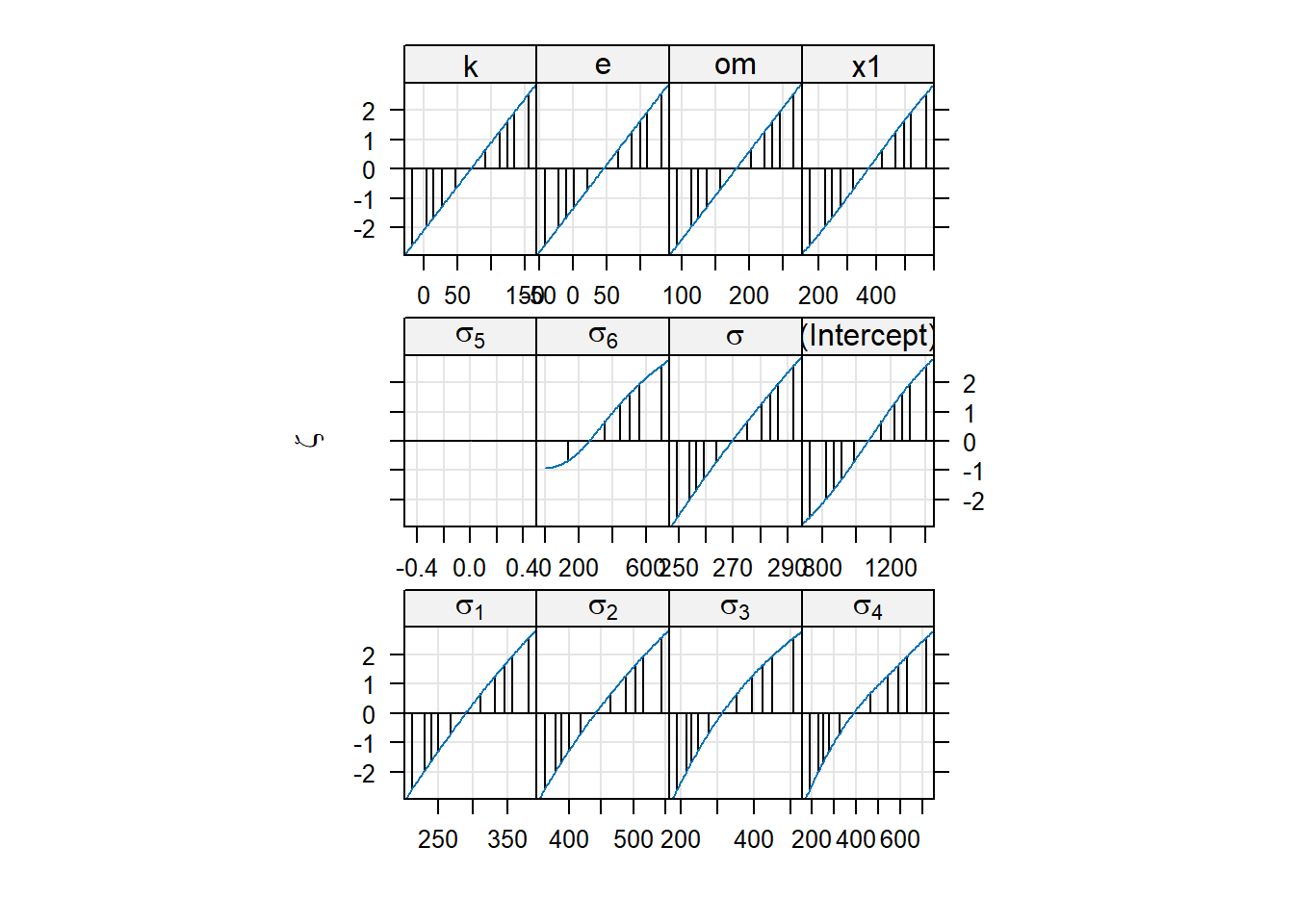
We can see that there are problems with the profiles of some of the variance components. We can use the summary to check which are those:
summary(lmm1b)Linear mixed model fit by REML. t-tests use Satterthwaite's method [
lmerModLmerTest]
Formula:
estimated.grain.yield_kg_ha ~ k + e + om + x1 + (1 + x1 || district/year/farm_id)
Data: pke.dat
REML criterion at convergence: 11476.8
Scaled residuals:
Min 1Q Median 3Q Max
-2.9298 -0.5216 -0.0490 0.4812 3.6955
Random effects:
Groups Name Variance Std.Dev.
farm_id.year.district x1 83251 288.5
farm_id.year.district.1 (Intercept) 194609 441.1
year.district x1 98602 314.0
year.district.1 (Intercept) 150370 387.8
district x1 5183 72.0
district.1 (Intercept) 82701 287.6
Residual 73039 270.3
Number of obs: 780, groups:
farm_id:year:district, 130; year:district, 26; district, 13
Fixed effects:
Estimate Std. Error df t value Pr(>|t|)
(Intercept) 1066.48 119.49 12.28 8.925 1.02e-06 ***
k 68.88 33.52 526.38 2.055 0.040382 *
e 44.09 33.52 526.38 1.315 0.188991
om 179.41 33.52 526.38 5.352 1.30e-07 ***
x1 371.01 76.64 11.51 4.841 0.000456 ***
---
Signif. codes: 0 '***' 0.001 '**' 0.01 '*' 0.05 '.' 0.1 ' ' 1
Correlation of Fixed Effects:
(Intr) k e om
k 0.000
e 0.000 -0.500
om 0.000 0.000 -0.500
x1 -0.035 -0.219 0.000 0.000We can see that the estimates of the variance components for district are the ones where there seems to be some estimation problems. Note that this is the factor that sits on top of the hierarchy and therefore it is the one that has the most uncertainty associated with it. This is a common problem with nested random effects, where the top level of the hierarchy is the one that is most difficult to estimate.
- We can check the normality of the residuals using a QQ plot:
qqnorm(resid(lmm1b))
qqline(resid(lmm1b))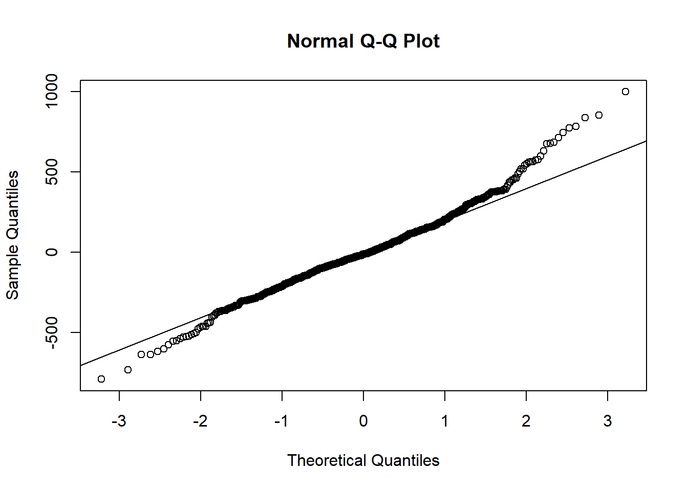
We see strong deviations from normality in the tails of the distribution. We can also use the plot function on the model object to check the homoscedasticity of the residuals:
plot(lmm1b)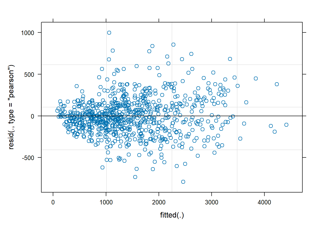
We can see that the residuals are not homoscedastic, there is a funnel effect where the variance is smaller at the lower end of the fitted values and larger at the higher end.
Let’s extract the variance components and show the contribution of each of these components to the total variance. First we extract the variance components and remove the correlation terms if present:
VC <- as.data.frame(VarCorr(lmm1b))
VC <- VC[is.na(VC$var2),]The sum of the variance components (including residuals) should match the variance of the data:
c(sum(VC$vcov), var(pke.dat$estimated.grain.yield_kg_ha))[1] 687755.8 752353.8We can see that is close enough (about 91% of the variance of the data). The mismatch is due to the fact that the variance components are estimated with some uncertainty, so the value sum(VC$vcov) actually has an uncertainty associated to it. Also, in general, estimates of variances tend to be biased downwards (the bias becomes smaller as the sample size increases).
We can visualize the contribution of each of the variance components to the total variance using a bar plot:
# make table with response variances
vc=VC$vcov
names(vc)<-paste(VC$grp,VC$var1) #set names to intercept/slope variance components
# make proportions
vc.prop<-vc/sum(vc)
# #order by (decreasing size)
vc.prop<-vc.prop[order(vc.prop, decreasing=T)]
# now plot
par_default <- par(no.readonly = TRUE) #save default parameters
par(mar=c(14,4,2,2)) #increase lower margin
barplot(vc.prop,las=2)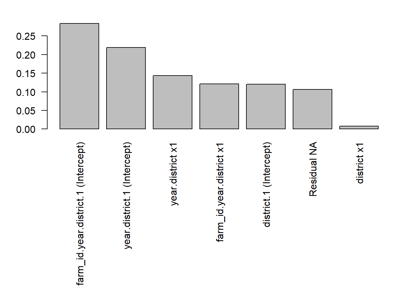
par(par_default) #reset to defaultWe can see that the farm and year components are the ones that contribute the most to the total variance, suggesting that there is substantial variation across farms and years in the effect of P fertilizer on yield.
To check on this, we can create subsets per district and year and fit separate models to compare the effects of P fertilizer. For example, let’s fit farm-level models to the data from Igabi and Kajuru districts in 2015:
dat.igabi.15 <- pke.dat[pke.dat$district == "igabi" & pke.dat$year == 2015,]
dat.kajuru.15 <- pke.dat[pke.dat$district == "kajuru" & pke.dat$year == 2015,]
lmm2.a<-lmer(estimated.grain.yield_kg_ha~k+e+om+x1+(1|farm_id),data=dat.igabi.15)
anova(lmm2.a)Type III Analysis of Variance Table with Satterthwaite's method
Sum Sq Mean Sq NumDF DenDF F value Pr(>F)
k 8109 8109 1 21 0.2110 0.6507
e 3071 3071 1 21 0.0799 0.7802
om 55042 55042 1 21 1.4323 0.2447
x1 20728 20728 1 21 0.5394 0.4708lmm2.b<-lmer(estimated.grain.yield_kg_ha~k+e+om+x1+(1|farm_id),data= dat.kajuru.15)
anova(lmm2.b)Type III Analysis of Variance Table with Satterthwaite's method
Sum Sq Mean Sq NumDF DenDF F value Pr(>F)
k 227571 227571 1 21 0.7212 0.405342
e 230157 230157 1 21 0.7294 0.402731
om 4034 4034 1 21 0.0128 0.911051
x1 3456966 3456966 1 21 10.9549 0.003333 **
---
Signif. codes: 0 '***' 0.001 '**' 0.01 '*' 0.05 '.' 0.1 ' ' 1We can see that in Kajuru the effect of P fertlizer on yield is significant, while in Igabi it is not.
Exercise 6.4
Extract the covariance matrix of the best model (
lmm1b) and visualize it. Explain the structure of the covariance matrix in relation to the data structureCompute the estimates of the coefficients and their standard errors using the linear algebra expressions we have taught you in the course (for fixed effects using the covariance matrix, the design matrix and the response variable).
Solution 6.4
- We can extract the covariance matrix and visualize it as follows:
V = getV(lmm1b)
image(V[1:70,1:70])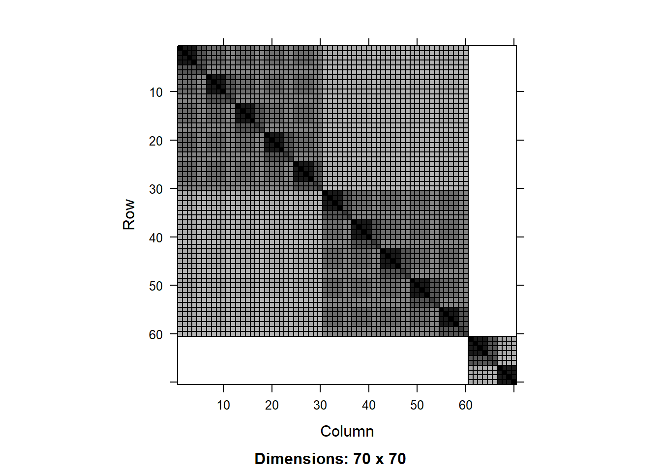
We can see a more complex structure of nested blocks of observations representing the different groups in the hierarchy. The big block of 60x60 represents the first district (bagwai, check table(pke.dat$district)), the two subblocks of 30x30 represent the two years (2015 and 2016), and the smaller blocks represent the farms.
- We extract the design matrix and the vector of response variables:
X <- model.matrix(lmm1b)
y <- pke.dat$estimated.grain.yield_kg_haWe apply the formulae to calculate the estimates of the coefficients and their standard errors:
# Estimates of coefficients
V_inv <- solve(V)
coef <- solve(t(X)%*%V_inv%*%X)%*%t(X)%*%V_inv%*%y
coef5 x 1 Matrix of class "dgeMatrix"
[,1]
(Intercept) 1066.47696
k 68.88258
e 44.08957
om 179.41296
x1 371.01233# Standard errors
COV <- solve(t(X)%*%V_inv%*%X)
SE <- sqrt(diag(COV))
SE(Intercept) k e om x1
119.48965 33.52122 33.52122 33.52122 76.63864 Compare to the output of the summary function:
summary(lmm1b)Linear mixed model fit by REML. t-tests use Satterthwaite's method [
lmerModLmerTest]
Formula:
estimated.grain.yield_kg_ha ~ k + e + om + x1 + (1 + x1 || district/year/farm_id)
Data: pke.dat
REML criterion at convergence: 11476.8
Scaled residuals:
Min 1Q Median 3Q Max
-2.9298 -0.5216 -0.0490 0.4812 3.6955
Random effects:
Groups Name Variance Std.Dev.
farm_id.year.district x1 83251 288.5
farm_id.year.district.1 (Intercept) 194609 441.1
year.district x1 98602 314.0
year.district.1 (Intercept) 150370 387.8
district x1 5183 72.0
district.1 (Intercept) 82701 287.6
Residual 73039 270.3
Number of obs: 780, groups:
farm_id:year:district, 130; year:district, 26; district, 13
Fixed effects:
Estimate Std. Error df t value Pr(>|t|)
(Intercept) 1066.48 119.49 12.28 8.925 1.02e-06 ***
k 68.88 33.52 526.38 2.055 0.040382 *
e 44.09 33.52 526.38 1.315 0.188991
om 179.41 33.52 526.38 5.352 1.30e-07 ***
x1 371.01 76.64 11.51 4.841 0.000456 ***
---
Signif. codes: 0 '***' 0.001 '**' 0.01 '*' 0.05 '.' 0.1 ' ' 1
Correlation of Fixed Effects:
(Intr) k e om
k 0.000
e 0.000 -0.500
om 0.000 0.000 -0.500
x1 -0.035 -0.219 0.000 0.000