library(rstan)
library(brms)
example(stan_model, package = "rstan", run.dontrun = TRUE)
brm(mpg~hp, data = mtcars)11 Bayesian inference: Linear and non-linear mixed models
In this practical we will work with the package brms to do Bayesian regression modelling. In the first half we will revisit some of the examples we have already gone through in the course. In the second half we will focus on non-linear mixed effect models using an example from photosynthesis research. No exercises are given in this chapter but the reader is motivated to try repeating some of the exercises in previous chapters with brms.
11.1 Setting up brms
The acronym brms stands for Bayesian Regression Modellin with Stan. Stan is the a probabilistic modelling language in C++ designed for Bayesian inference. What brms offers is a formula interface following similar syntax to other R functions such as lm, glm, or lmer. Models specified in brms are then translated to Stan, compiled and ran such that the user does not need to interact with the C++ probabilistic language.
Installing and setting up brms can be tricky. For that reason, there is an option to run this chapter without actually executing the Stan code but rather loading the result of fitting the models from RDS object. However, I still encourage you to setup brms properly in your computer so that you can run your own Bayesian model.
There are two interfaces in R to Stan: rstan and cmdstanr. The former has less functionality and is being phased out as the Stan development focuses mostly on cmdstanr. However, it might be easier to install and setup rstan in your computer. I give you instructions on how to setup both packages in your computer, assuming you are using Windows (for other platforms please check https://learnb4ss.github.io/learnB4SS/articles/install-brms.html or other sources online).
11.1.1 Using brms and rstan
Please follow these steps to install rstan and brms:
- Install Rtools 4.4. (https://cran.r-project.org/bin/windows/Rtools/)
- Install brms and rstan using the typical procedure
- Check that it works by running the following code:
11.1.2 Using brms and cmdstanr
Setting up cmdstanr is more complicated. Please follow these steps:
- Install Rtools 4.4. (https://cran.r-project.org/bin/windows/Rtools/)
- If you have R or RStudio open, please close it.
- Open rtools44 Bash (from the start menu in Windows)
- Run
pacman -Syu mingw-w64-x86_64-makein that Bash terminal you just opened. Say yes to all the questions. - Open R or Rstudio and run the command
install.packages("cmdstanr", repos = c('https://stan-dev.r-universe.dev', getOption("repos")))
cmdstanr::install_cmdstan(overwrite=TRUE)- Install brms as usual and test that it works by running the following code:
library(cmdstanr)
library(brms)
brm(mpg~hp, data = mtcars, backend = "cmdstanr")
11.1.3 Common setup for this chapter
Make sure you run this code at the start of the script:
library(brms)
library(rstan) # We still need for some functions even if cmdstanr is installed
library(cmdstanr) # If you are using it
options(mc.cores = parallel::detectCores()) # To run in parallel
RUN = FALSE # Change to TRUE to run the code
If you want to could not setup rstan or cmdstanr you can set RUN = FALSE and that will avoid running the code that fits the models. Instead, it will load the results from RDS files that I have already generated. You can find these files in the data/processed folder.
Even if you can run the code, I recommend to set RUN = FALSE for the second half on non-linear mixed models as the last two models take a long time to run (the most complex model took an hour to fit on my computer!).
11.2 Linear (mixed) models in brms
In this first section we are going to fit some simple linear and mixed models using brms and compared them to the classical approach using lm and lmer. We will learn how to specify priors and how to analyze the results of a Bayesian model. Note that this is only illustrating a small subset of all the functionality of brms (which actually covers all the types of models that we have seen in the course, and beyond) but it easier to learn the workflow and basic concepts with simpler examples.
11.2.1 A simple linear model
We are going to start with a simpler linear model with one categorical predictor. We will use the iris dataset that is included in R by default. This dataset contains measurements of sepal length, sepal width, petal length and petal width for three species of iris flowers (it was originally used by Fisher to introduce a classification technique):
head(iris) Sepal.Length Sepal.Width Petal.Length Petal.Width Species
1 5.1 3.5 1.4 0.2 setosa
2 4.9 3.0 1.4 0.2 setosa
3 4.7 3.2 1.3 0.2 setosa
4 4.6 3.1 1.5 0.2 setosa
5 5.0 3.6 1.4 0.2 setosa
6 5.4 3.9 1.7 0.4 setosaWe are going to model the effects of species on sepal length using the dataset iris. The formula for this model is Sepal.Length~Species. We can fit this model using brms as by calling the function brm with the formula and the data as arguments:
if(RUN) {
    fit <- brm(Sepal.Length~Species, data = iris, backend = "cmdstanr",
               save_model = "stan/iris", seed = 1234)
} else {
    fit <- readRDS("data/processed/fit_iris.rds")
}
#saveRDS(fit, "data/processed/fit_iris.rds")
The argument save_model will save the model as a file such that it does not need to be recompiled again every time you want to run it (if you use "cmdstanr" as the backend). The seed argument is to make sure that the results are reproducible (despite using a Monte Carlo approach).
A summary of the model gives information about the parameter estimates and convergence of the numerical algorithm:
summary(fit) Family: gaussian
Links: mu = identity; sigma = identity
Formula: Sepal.Length ~ Species
Data: iris (Number of observations: 150)
Draws: 4 chains, each with iter = 2000; warmup = 1000; thin = 1;
total post-warmup draws = 4000
Regression Coefficients:
Estimate Est.Error l-95% CI u-95% CI Rhat Bulk_ESS Tail_ESS
Intercept 5.00 0.07 4.86 5.15 1.00 3377 2880
Speciesversicolor 0.93 0.10 0.74 1.13 1.00 3447 2880
Speciesvirginica 1.58 0.10 1.38 1.79 1.00 3692 3302
Further Distributional Parameters:
Estimate Est.Error l-95% CI u-95% CI Rhat Bulk_ESS Tail_ESS
sigma 0.52 0.03 0.46 0.58 1.00 3629 2755
Draws were sampled using sample(hmc). For each parameter, Bulk_ESS
and Tail_ESS are effective sample size measures, and Rhat is the potential
scale reduction factor on split chains (at convergence, Rhat = 1).These estimates are analogous to the ones we would obtain with lm. In terms of checking convergence we want to make sure that Rhat is below 1.10 and that Tail_ESS is in the thousands (this determines how accurate the estimates of means and 95% intervals are).
Compare these results to the classical frequentist:
fit_classic <- lm(Sepal.Length~Species, data = iris)
summary(fit_classic)
Call:
lm(formula = Sepal.Length ~ Species, data = iris)

Residuals:
    Min      1Q  Median      3Q     Max
-1.6880 -0.3285 -0.0060  0.3120  1.3120

Coefficients:
                  Estimate Std. Error t value Pr(>|t|)
(Intercept)         5.0060     0.0728  68.762  < 2e-16 ***
Speciesversicolor   0.9300     0.1030   9.033 8.77e-16 ***
Speciesvirginica    1.5820     0.1030  15.366  < 2e-16 ***
---
Signif. codes:  0 '***' 0.001 '**' 0.01 '*' 0.05 '.' 0.1 ' ' 1

Residual standard error: 0.5148 on 147 degrees of freedom
Multiple R-squared:  0.6187,    Adjusted R-squared:  0.6135
F-statistic: 119.3 on 2 and 147 DF,  p-value: < 2.2e-16
The estimates are pratically the same. What priors did brms use? We can see this by using the function default_prior:
default_prior(Sepal.Length~Species, data = iris) prior class coef group resp dpar nlpar lb ub
(flat) b
(flat) b Speciesversicolor
(flat) b Speciesvirginica
student_t(3, 5.8, 2.5) Intercept
student_t(3, 0, 2.5) sigma 0
source
default
(vectorized)
(vectorized)
default
defaultThese are weakly informative priors (scaled by your data) for the intercept but flat prior for the effects. The parameters associated to fixed effects are denoted with class = "b", the intercept with class = "Intercept" and the residual standard deviation with class = "sigma". One can assign separate priors to each of the fixed effects or a common prior to all of them (that is why there are multiple entries for class b).
11.2.1.1 Weakly informative priors
The general recommendation in modern Bayesian data analysis is to always use weakly informative priors (WIPs) unless you have prior information that can be justified scientifically. The procedure to use WIPs is as follows:
- Standardize (or scale) the response variables and any continuous predictor.
- Choose the level of shrinkage that we want to achieve with the WIP.
- Assign priors as reference distributions (often centered at 0) with a spread that is determined by point 2 (the more informative the less spread).
Point 2 and 3 are a bit unspecified and there are different guidelines that could be follow. I could not find specific WIP guidelines for agricultural research (they use of Bayesian statistics in agronomy is in its toddler stage) but I will borrow guidelines from other fields (e.g., https://par.nsf.gov/servlets/purl/10106121 or https://github.com/stan-dev/stan/wiki/Prior-Choice-Recommendations).
Let’s first scale the response variable (this means substracting the mean and dividing by the standard deviation):
iris$Sepal.Length.Scaled <- scale(iris$Sepal.Length)Now we will specify the following priors:
- For intercept and fixed effects: Normal(0,1)
- For standard deviation: Normal(0,2.5) (technically half distributions because the parameter is positive).
Note: If you do not want to scale the variables you could try Normal(mu, sigma) for intercept and N(0, sigma) for effects where mu and sigma are the means and standard deviations of the response variable. However, this approach does not generalize to more complex models (e.g., for slopes it would depend on the scales of the prediction and response variable, as well as for interactions involving continuous predictors).
We can assign priors in brms as follows. Note that we should specify that the standard deviation is positive (i.e., larger than 0) using the lb argument. We are using strings to specify the priors but there are other formats available in brms:
priors <- c(prior("normal(0,1)", class = "b", coef = "Speciesversicolor"),
            prior("normal(0,1)", class = "b", coef = "Speciesvirginica"),
            prior("normal(0,1)", class = "Intercept"),
            prior("normal(0,2.5)", class = "sigma", lb = 0))
priors
prior class coef group resp dpar nlpar lb ub
normal(0,1) b Speciesversicolor <NA> <NA>
normal(0,1) b Speciesvirginica <NA> <NA>
normal(0,1) Intercept <NA> <NA>
normal(0,2.5) sigma 0 <NA>
source
user
user
user
userWe can now fit the model with these new priors (and I will redo the original fit with the scaled response for comparison):
if(RUN) {
    fit_WIP <- brm(Sepal.Length.Scaled~Species, data = iris, backend = "cmdstanr",
                save_model = "stan/iris_WIP", seed = 1234, prior = priors)
    fit_scaled <- brm(Sepal.Length.Scaled~Species, data = iris, backend = "cmdstanr",
                save_model = "stan/iris_scaled", seed = 1234)
} else {
    fit_WIP <- readRDS("data/processed/fit_iris_WIP.rds")
    fit_scaled <- readRDS("data/processed/fit_iris_scaled.rds")
}
#saveRDS(fit_WIP, "data/processed/fit_iris_WIP.rds")
#saveRDS(fit_scaled, "data/processed/fit_iris_scaled.rds")
Let’s quickly compare the three approaches:
fixef(fit_scaled) Estimate Est.Error Q2.5 Q97.5
Intercept -1.012256 0.08706992 -1.1859243 -0.8437751
Speciesversicolor 1.124382 0.12541264 0.8766959 1.3654647
Speciesvirginica 1.912146 0.12625287 1.6605493 2.1638382fixef(fit_WIP) Estimate Est.Error Q2.5 Q97.5
Intercept -0.9899175 0.08666026 -1.1602010 -0.8171362
Speciesversicolor 1.0953299 0.12362292 0.8550535 1.3320760
Speciesvirginica 1.8744862 0.12183321 1.6353185 2.1113590summary(lm(Sepal.Length.Scaled~Species, data = iris))
Call:
lm(formula = Sepal.Length.Scaled ~ Species, data = iris)

Residuals:
     Min       1Q   Median       3Q      Max
-2.03848 -0.39671 -0.00725  0.37678  1.58441

Coefficients:
                  Estimate Std. Error t value Pr(>|t|)
(Intercept)       -1.01119    0.08792 -11.501  < 2e-16 ***
Speciesversicolor  1.12310    0.12434   9.033 8.77e-16 ***
Speciesvirginica   1.91048    0.12434  15.366  < 2e-16 ***
---
Signif. codes:  0 '***' 0.001 '**' 0.01 '*' 0.05 '.' 0.1 ' ' 1

Residual standard error: 0.6217 on 147 degrees of freedom
Multiple R-squared:  0.6187,    Adjusted R-squared:  0.6135
F-statistic: 119.3 on 2 and 147 DF,  p-value: < 2.2e-16
You can see that the estimates are pratically the same, with somewhat smaller estimates for the effects of species (but well within the uncertainty!). In both cases the estimates also coincide with the classic estimates. Remember that for the Bayesian estimate we are using the mean of the posterior distribution as a point estimate (but the real Bayesian estimate is the whole posterior distribution).
We can visualize how Bayes rule has updated the estimates of parameters (from prior to posterior). Below I plot the priors from the WIP approach and the posterior for both models (WIP and default brms choice):
posterior_WIP <- as_draws_df(fit_WIP)
posterior_scaled <- as_draws_df(fit_scaled)
par(mfrow = c(2,2))
plot(density(posterior_WIP$Intercept), main = "Intercept (Setosa)", ylab = "Density", xlab = "")
lines(density(posterior_scaled$Intercept), col = "grey", lty = 2)
curve(dnorm(x, 0, 1), add = TRUE, col = 2)
plot(density(posterior_WIP$b_Speciesversicolor), main = "Versicolor", ylab = "Density", xlab = "")
lines(density(posterior_scaled$b_Speciesversicolor), col = "grey", lty = 2)
curve(dnorm(x, 0, 1), add = TRUE, col = 2)
plot(density(posterior_WIP$b_Speciesvirginica), main = "Virginica", ylab = "Density", xlab = "")
lines(density(posterior_scaled$b_Speciesvirginica), col = "grey", lty = 2)
curve(dnorm(x, 0, 1), add = TRUE, col = 2)
plot(density(posterior_WIP$sigma), main = "sd", ylab = "Density", xlab = "")
lines(density(posterior_scaled$sigma), col = "grey", lty = 2)
curve(dnorm(x, 0, 2.5), add = TRUE, col = 2)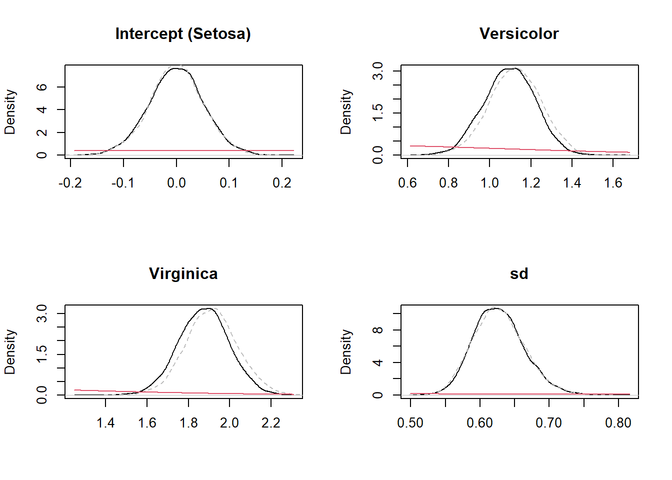
par(mfrow = c(1,1))You can see that (i) the prior distribution is practically flat in the range of values that we see in the posterior distribution (so it does not affect its shape much) such that both approaches have yielded practically the same posteriors. Of course this will not alwaus be the case.
11.2.1.2 Bayesian hypothesis testing
We can test hypothesis associated to specific constrats (one sided) with the hypothesis function. For example, I can see that the effects of species is estimated to be positive. I would like to test that indeed that is case. I can do it as follows:
hypothesis(fit_WIP, c("Speciesversicolor > 0", "Speciesvirginica > 0"))Hypothesis Tests for class b:
Hypothesis Estimate Est.Error CI.Lower CI.Upper Evid.Ratio
1 (Speciesversicolor) > 0 1.10 0.12 0.89 1.29 Inf
2 (Speciesvirginica) > 0 1.87 0.12 1.67 2.08 Inf
Post.Prob Star
1 1 *
2 1 *
---
'CI': 90%-CI for one-sided and 95%-CI for two-sided hypotheses.
'*': For one-sided hypotheses, the posterior probability exceeds 95%;
for two-sided hypotheses, the value tested against lies outside the 95%-CI.
Posterior probabilities of point hypotheses assume equal prior probabilities.There are two types of tests being done:
The probability that the coefficients are larger than 0 divided by the probability that is smaller than 0. This is the evidence ratio (we did not have any samples below 0 so it is actually Inf, in practice it means an overwhelming evidence in favour of our hypothesis).
The posterior probability of the hypothesis being true (in this case 1 because all the posterior was above 0).
We can have arbitrarily complex hypotheses (e.g., that the difference between versicolor and setosa, the reference level, is larger than 1 standard deviation):
hypothesis(fit_WIP, "Speciesversicolor > 1")Hypothesis Tests for class b:
Hypothesis Estimate Est.Error CI.Lower CI.Upper Evid.Ratio
1 (Speciesversicolo... > 0 0.1 0.12 -0.11 0.29 3.56
Post.Prob Star
1 0.78
---
'CI': 90%-CI for one-sided and 95%-CI for two-sided hypotheses.
'*': For one-sided hypotheses, the posterior probability exceeds 95%;
for two-sided hypotheses, the value tested against lies outside the 95%-CI.
Posterior probabilities of point hypotheses assume equal prior probabilities.Here we see that the probability of the effect being larger than 1 standar deviation (almost 80%) and the evidence ratio is larger than 1. This is not however as overwhelming as the previous hypotheses. If we keep the 95% as the magic number for statistical decisions we would say that this experiment (plus our model and prior assumptions about possible effect sizes) does not show sufficient evidence to support the second hypothesis. Of course, the 95% is arbitrary and in some contexts you may want to accept smaller evidence or even make the requirements stricter.
We can build a nested model (without Species) and use model comparison to test where Species has any influence on Sepal.Length:
if(RUN) {
    null_fit <- brm(Sepal.Length.Scaled~1, data = iris, backend = "cmdstanr", save_model = "stan/iris_null",
                    prior = c(prior("normal(0,1)", class = "Intercept"),
                              prior("normal(0,2.5)", class = "sigma", lb = 0)))
} else {
    null_fit <- readRDS("data/processed/null_iris_fit.rds")
}
#saveRDS(null_fit, "data/processed/null_iris_fit.rds")
We can compare the models using leave-one-out cross validation (LOO):
loo(fit_WIP, null_fit)Output of model 'fit_WIP':
Computed from 4000 by 150 log-likelihood matrix.
Estimate SE
elpd_loo -144.1 9.3
p_loo 4.0 0.7
looic 288.3 18.6
------
MCSE of elpd_loo is 0.0.
MCSE and ESS estimates assume MCMC draws (r_eff in [0.8, 1.2]).
All Pareto k estimates are good (k < 0.7).
See help('pareto-k-diagnostic') for details.
Output of model 'null_fit':
Computed from 4000 by 150 log-likelihood matrix.
Estimate SE
elpd_loo -214.2 7.3
p_loo 1.7 0.2
looic 428.5 14.7
------
MCSE of elpd_loo is 0.0.
MCSE and ESS estimates assume MCMC draws (r_eff in [0.7, 1.0]).
All Pareto k estimates are good (k < 0.7).
See help('pareto-k-diagnostic') for details.
Model comparisons:
elpd_diff se_diff
fit_WIP 0.0 0.0
null_fit -70.1 8.4 We see that the elpd (expected log probability density) is highest for the larger model and the different is quite large (more than 10 times the standard error of the elpd estimate).
Stringly speaking this only means that including Species improves the predictive accuracy of the model. In practice it may be used as a form of null hypothesis testing just like a likelihood ratio test. The recommendations then is to only consider differences in elpd larger than 4 and when the difference is larger than twice its standard error. Thus in this case we would conclude that Species has a clear effect on sepal length and (at least as statistics is concerned) worth including in the model.
11.2.1.3 Marginal means
We can also calculate marginal means
library(emmeans)
marginal_means <- emmeans(fit_WIP, "Species")
marginal_means
Species emmean lower.HPD upper.HPD
setosa -0.990 -1.1662 -0.825
versicolor 0.105 -0.0693 0.281
virginica 0.885 0.7183 1.061
Point estimate displayed: median
HPD interval probability: 0.95 Of course these means are not in the original scale. You can backtransform to the original scale:
mu = mean(iris$Sepal.Length)
sigma = sd(iris$Sepal.Length)
posterior_WIP$Sepal.Length.Setosa <- posterior_WIP$Intercept*sigma + mu
posterior_WIP$Sepal.Length.Versicolor <- (posterior_WIP$Intercept + posterior_WIP$b_Speciesversicolor)*sigma + mu
posterior_WIP$Sepal.Length.Virginica <- (posterior_WIP$Intercept + posterior_WIP$b_Speciesvirginica)*sigma + mu
And just summarize them yourself (e.g., we can compute a 95% interval and the median with the quantile function, just to emphasize that choosing the mean is not the only option):
with(posterior_WIP, rbind(setosa = quantile(Sepal.Length.Setosa, c(0.025, 0.5, 0.975)),
                          versicolor = quantile(Sepal.Length.Versicolor, c(0.025, 0.5, 0.975)),
                          virginica = quantile(Sepal.Length.Virginica, c(0.025, 0.5, 0.975))))
2.5% 50% 97.5%
setosa 5.757953 5.843491 5.926744
versicolor 6.522447 6.749999 6.965343
virginica 7.176046 7.397489 7.61147711.2.1.4 Small samples
We have shown above that the results are the same for classic and Bayesian estimate with uninformative priors and (practically the same) for the version with WIP. However we had a rather uncommon situation: a model with 4 parameters (intercept, two effects plus residual variance) and 150 data points. This is in the domain of “large samples” (i.e., n/k > 30) where, indeed, the results from Bayesian and classical analysis converge to each other (unless the priors are very informative and contradict the likelihood). A more realistic example is when the sample size is small. Let’s subset the iris dataset such that we only have five replicates per group:
iris_small <- iris[c(1:5, 51:55, 101:105),]
iris_small
Sepal.Length Sepal.Width Petal.Length Petal.Width Species
1 5.1 3.5 1.4 0.2 setosa
2 4.9 3.0 1.4 0.2 setosa
3 4.7 3.2 1.3 0.2 setosa
4 4.6 3.1 1.5 0.2 setosa
5 5.0 3.6 1.4 0.2 setosa
51 7.0 3.2 4.7 1.4 versicolor
52 6.4 3.2 4.5 1.5 versicolor
53 6.9 3.1 4.9 1.5 versicolor
54 5.5 2.3 4.0 1.3 versicolor
55 6.5 2.8 4.6 1.5 versicolor
101 6.3 3.3 6.0 2.5 virginica
102 5.8 2.7 5.1 1.9 virginica
103 7.1 3.0 5.9 2.1 virginica
104 6.3 2.9 5.6 1.8 virginica
105 6.5 3.0 5.8 2.2 virginica
Sepal.Length.Scaled
1 -0.89767388
2 -1.13920048
3 -1.38072709
4 -1.50149039
5 -1.01843718
51 1.39682886
52 0.67224905
53 1.27606556
54 -0.41462067
55 0.79301235
101 0.55148575
102 -0.05233076
103 1.51759216
104 0.55148575
105 0.79301235Let’s now fit all the models used above:
iris_small$Sepal.Length.Scaled <- scale(iris_small$Sepal.Length)
if(RUN) {
    fit_WIP <- brm(Sepal.Length.Scaled~Species, data = iris_small, backend = "cmdstanr",
                save_model = "stan/iris_small_WIP", seed = 1234, prior = priors)
    fit_scaled <- brm(Sepal.Length.Scaled~Species, data = iris_small, backend = "cmdstanr",
                save_model = "stan/iris_small_scaled", seed = 1234)
    null_fit <- brm(Sepal.Length.Scaled~1, data = iris_small, backend = "cmdstanr",
                    save_model = "stan/iris_small_null", prior = c(prior("normal(0,1)",
                    class = "Intercept"), prior("normal(0,2.5)", class = "sigma", lb = 0)))
} else {
    fit_WIP <- readRDS("data/processed/fit_iris_small_WIP.rds")
    fit_scaled <- readRDS("data/processed/fit_iris_small_scaled.rds")
    null_fit <- readRDS("data/processed/fit_iris_small_null.rds")
}
#saveRDS(fit_WIP, "data/processed/fit_iris_small_WIP.rds")
#saveRDS(fit_scaled, "data/processed/fit_iris_small_scaled.rds")
#saveRDS(null_fit, "data/processed/fit_iris_small_null.rds")
fit_classic <- lm(Sepal.Length.Scaled~Species, data = iris_small)
Let’s look at the coefficients:
fixef(fit_scaled) Estimate Est.Error Q2.5 Q97.5
Intercept -1.195994 0.2616671 -1.720256 -0.6594225
Speciesversicolor 1.822353 0.3659389 1.096733 2.5591393
Speciesvirginica 1.767428 0.3732374 1.046717 2.4965437fixef(fit_WIP) Estimate Est.Error Q2.5 Q97.5
Intercept -0.9766587 0.2695571 -1.4571125 -0.3809078
Speciesversicolor 1.4958319 0.3758181 0.6719691 2.1759005
Speciesvirginica 1.4424993 0.3712494 0.6364896 2.0953598summary(fit_classic)
Call:
lm(formula = Sepal.Length.Scaled ~ Species, data = iris_small)

Residuals:
     Min       1Q   Median       3Q      Max
-1.09865 -0.14878  0.04578  0.21744  0.80110

Coefficients:
                  Estimate Std. Error t value Pr(>|t|)
(Intercept)        -1.1978     0.2319  -5.165 0.000235 ***
Speciesversicolor   1.8311     0.3280   5.583 0.000119 ***
Speciesvirginica    1.7624     0.3280   5.374 0.000167 ***
---
Signif. codes:  0 '***' 0.001 '**' 0.01 '*' 0.05 '.' 0.1 ' ' 1

Residual standard error: 0.5186 on 12 degrees of freedom
Multiple R-squared:  0.7695,    Adjusted R-squared:  0.7311
F-statistic: 20.03 on 2 and 12 DF,  p-value: 0.00015
We can see that the estimates are again quite similar between the model with flat priors and the classic method (notice that the standard errors are a bit higher for the Bayesian estimate). The model with WIP has a larger intercept and smaller effect sizes though again this is well within the uncertainty.
Let’s compare again the prior and posterior distributions:
posterior_WIP <- as_draws_df(fit_WIP)
posterior_scaled <- as_draws_df(fit_scaled)
par(mfrow = c(2,2))
plot(density(posterior_WIP$Intercept), main = "Intercept (Setosa)", ylab = "Density", xlab = "")
lines(density(posterior_scaled$Intercept), col = "grey", lty = 2)
curve(dnorm(x, 0, 1), add = TRUE, col = 2)
plot(density(posterior_WIP$b_Speciesversicolor), main = "Versicolor", ylab = "Density", xlab = "")
lines(density(posterior_scaled$b_Speciesversicolor), col = "grey", lty = 2)
curve(dnorm(x, 0, 1), add = TRUE, col = 2)
plot(density(posterior_WIP$b_Speciesvirginica), main = "Virginica", ylab = "Density", xlab = "")
lines(density(posterior_scaled$b_Speciesvirginica), col = "grey", lty = 2)
curve(dnorm(x, 0, 1), add = TRUE, col = 2)
plot(density(posterior_WIP$sigma), main = "sd", ylab = "Density", xlab = "")
lines(density(posterior_scaled$sigma), col = "grey", lty = 2)
curve(dnorm(x, 0, 2.5), add = TRUE, col = 2)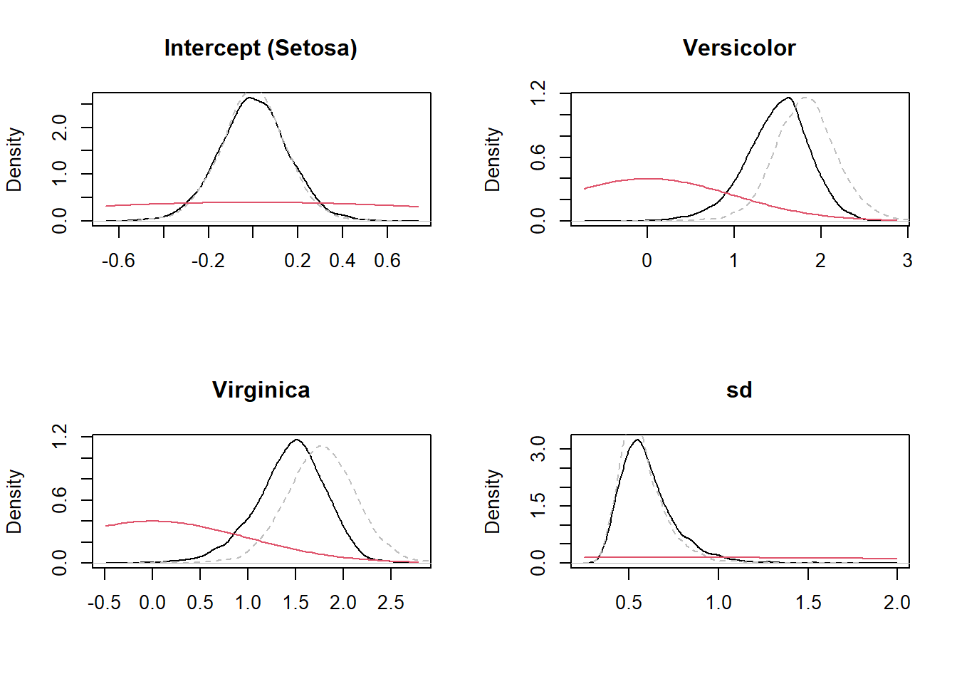
par(mfrow = c(1,1))You can see that for some of the parameters, the section of the prior that is relevant is no longer flat and in those cases we see a stronger shrinkage (i.e., the posterior under WIP is shifted with respect to the posterior under flat priors). Indeed, whether a prior is more or less informative depends on the model and data (especially sample size) and not just the prior itself. For large samples, the effect of priors is always diminished (so they become less informative) whereas for small samples all priors become more informative. The idea of WIP is that they do not dominate the estimate even for small data (as in this example) and that they tend to shrink effect sizes towards zero (making the estimates more conservative, reducing false positive errors in hypothesis testing).
Notice how the posterior distribution of the residual standard deviation is highly skewed and not symmetric. This is because the standard deviation is a constrained variable (it cannot be negative) and the uncertainty about it is quite large. We saw in the summary before that the estimates reported by brms are larger than in the classical approach. However, this is mostly because we are reporting means of the posterior distribution. If we calculate the median and the mode we can see why it is important to remember that the Bayesian estimate is the entire distribution and not just the mean:
library(bayestestR)
mean(posterior_WIP$sigma) # 0.60
[1] 0.6040078median(posterior_WIP$sigma) # 0.57[1] 0.574973map_estimate(posterior_WIP$sigma)[1,2] # 0.55[1] 0.5464825sigma(fit_classic) # 0.52[1] 0.5185832plot(density(posterior_WIP$sigma), ylab = "Density", xlab = "sigma", main = "",
xlim = c(0, 1.3))
abline(v = sigma(fit_classic), col = "red", lty = 1)
abline(v = mean(posterior_WIP$sigma), col = "blue", lty = 2)
abline(v = median(posterior_WIP$sigma), col = "green", lty = 3)
abline(v = map_estimate(posterior_WIP$sigma)[1,2], col = "purple", lty = 4)
abline(v = quantile(posterior_WIP$sigma, c(0.025, 0.975)), col = "lightgray")
legend("topright",
legend = c("Classical","Mean", "Median", "Mode"),
col = c("red", "blue", "green", "purple"),
lty = 1:4)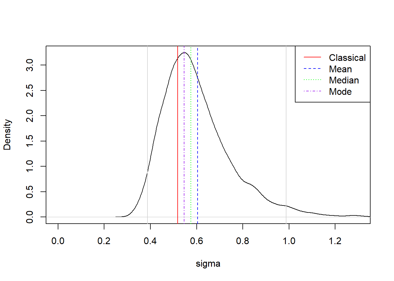
Let’s test the same hypotheses as before:
hypothesis(fit_WIP, c("Speciesversicolor > 0", "Speciesvirginica > 0"))Hypothesis Tests for class b:
Hypothesis Estimate Est.Error CI.Lower CI.Upper Evid.Ratio
1 (Speciesversicolor) > 0 1.50 0.38 0.85 2.07 1332.33
2 (Speciesvirginica) > 0 1.44 0.37 0.79 2.00 665.67
Post.Prob Star
1 1 *
2 1 *
---
'CI': 90%-CI for one-sided and 95%-CI for two-sided hypotheses.
'*': For one-sided hypotheses, the posterior probability exceeds 95%;
for two-sided hypotheses, the value tested against lies outside the 95%-CI.
Posterior probabilities of point hypotheses assume equal prior probabilities.We still have very storng evidence of a positive effect in sepal length. We can also test the effect of Species overall:
loo(fit_WIP, fit_scaled, null_fit)Warning: Found 1 observations with a pareto_k > 0.7 in model 'fit_WIP'. We
recommend to set 'moment_match = TRUE' in order to perform moment matching for
problematic observations.Warning: Found 1 observations with a pareto_k > 0.7 in model 'fit_scaled'. We
recommend to set 'moment_match = TRUE' in order to perform moment matching for
problematic observations.Output of model 'fit_WIP':
Computed from 4000 by 15 log-likelihood matrix.
Estimate SE
elpd_loo -15.1 2.8
p_loo 3.6 1.2
looic 30.1 5.7
------
MCSE of elpd_loo is NA.
MCSE and ESS estimates assume MCMC draws (r_eff in [0.4, 1.0]).
Pareto k diagnostic values:
Count Pct. Min. ESS
(-Inf, 0.7] (good) 14 93.3% 1070
(0.7, 1] (bad) 1 6.7% <NA>
(1, Inf) (very bad) 0 0.0% <NA>
See help('pareto-k-diagnostic') for details.
Output of model 'fit_scaled':
Computed from 4000 by 15 log-likelihood matrix.
Estimate SE
elpd_loo -14.4 3.2
p_loo 3.6 1.4
looic 28.9 6.4
------
MCSE of elpd_loo is NA.
MCSE and ESS estimates assume MCMC draws (r_eff in [0.5, 1.0]).
Pareto k diagnostic values:
Count Pct. Min. ESS
(-Inf, 0.7] (good) 14 93.3% 1125
(0.7, 1] (bad) 1 6.7% <NA>
(1, Inf) (very bad) 0 0.0% <NA>
See help('pareto-k-diagnostic') for details.
Output of model 'null_fit':
Computed from 4000 by 15 log-likelihood matrix.
Estimate SE
elpd_loo -22.4 1.4
p_loo 1.1 0.2
looic 44.8 2.8
------
MCSE of elpd_loo is 0.0.
MCSE and ESS estimates assume MCMC draws (r_eff in [0.6, 0.7]).
All Pareto k estimates are good (k < 0.7).
See help('pareto-k-diagnostic') for details.
Model comparisons:
elpd_diff se_diff
fit_scaled 0.0 0.0
fit_WIP -0.6 0.8
null_fit -8.0 3.6 According to the guidelines above, we would still conclude that Species has an effect on sepal length, though this is bit closer to the edge (difference is closer to 4 and barely bigger than twice the standard error). Note that it is also valid to compare models with different priors (as in the Bayesian world, the priors are part of the model!). Here we can see that the priors do not really matter much in terms of predictive power (for this case). I do not recommend to choose priors based on predictive power as that would imply your prior is (indirectly) determined by the data (but this has inspired certain practices in machine learning, called hyperparameter tuning, so when your goals are purely predictive this may be useful).
11.2.2 More complex model
Let’s revisit the nitrogen dataset from Chapter 2
dat <- read.csv("data/raw/Spacing and nitrogen_max225.csv", header = T)
dat$block <- factor(dat$block)
dat$Spacing <- factor(dat$Spacing, levels = c("less", "recommended", "more"))
dat$NitrogenF <- factor(dat$Nitrogen)
Let’s treat the block as a random effect and include the interactions between Nitrogen and Spacing. Which priors will it assume by default?
default_prior(Yield~NitrogenF*Spacing + (1 | block), data = dat) prior class coef group resp
(flat) b
(flat) b NitrogenF150
(flat) b NitrogenF150:Spacingmore
(flat) b NitrogenF150:Spacingrecommended
(flat) b NitrogenF225
(flat) b NitrogenF225:Spacingmore
(flat) b NitrogenF225:Spacingrecommended
(flat) b NitrogenF75
(flat) b NitrogenF75:Spacingmore
(flat) b NitrogenF75:Spacingrecommended
(flat) b Spacingmore
(flat) b Spacingrecommended
student_t(3, 47.8, 16.6) Intercept
student_t(3, 0, 16.6) sd
student_t(3, 0, 16.6) sd block
student_t(3, 0, 16.6) sd Intercept block
student_t(3, 0, 16.6) sigma
dpar nlpar lb ub source
default
(vectorized)
(vectorized)
(vectorized)
(vectorized)
(vectorized)
(vectorized)
(vectorized)
(vectorized)
(vectorized)
(vectorized)
(vectorized)
default
0 default
0 (vectorized)
0 (vectorized)
0 defaultAs before, we see flat prior over all fixed effects, but weakly informative priors (scaled by data) over the intercept and all the variance components. Let’s scale the response variable (the predictors are all categorical so nothing to scale there):
dat$YieldScaled <- scale(dat$Yield)And we can set our standard WIP distributions:
priors <- c(prior("normal(0,1)", class = "b"),
            prior("normal(0,1)", class = "Intercept"),
            prior("normal(0,2.5)", class = "sigma", lb = 0),
            prior("normal(0,2.5)", class = "sd", lb = 0))
priors
prior class coef group resp dpar nlpar lb ub source
normal(0,1) b <NA> <NA> user
normal(0,1) Intercept <NA> <NA> user
normal(0,2.5) sigma 0 <NA> user
normal(0,2.5) sd 0 <NA> userNote that we did not specify every individual coefficient, but rather the classes of coefficients (and this information will be automatically applied to all coefficients).
Let’s fit the model. This time I already calculated the elpd values from LOO so that I can use them later for model comparison:
if(RUN) {
    fit_NS <- brm(YieldScaled~NitrogenF*Spacing + (1 | block),
                data = dat, backend = "cmdstanr", prior = priors,
                save_model = "stan/NS", control = list(adapt_delta = 0.99)) |>
            add_criterion("loo")
} else {
    fit_NS <- readRDS("data/processed/fit_iris_NS.rds")
}
#saveRDS(fit_NS, "data/processed/fit_iris_NS.rds")
Because we are fitting a random effect with only 2 levels, I had to tune the MCMC to work a bit harder (this is done by increasing adapt_delta). I did this iteratively based on earlier runs. This increases the computation time but guarantees proper sampling. Let’s look at the output:
fit_NS Family: gaussian
Links: mu = identity; sigma = identity
Formula: YieldScaled ~ NitrogenF * Spacing + (1 | block)
Data: dat (Number of observations: 24)
Draws: 4 chains, each with iter = 2000; warmup = 1000; thin = 1;
total post-warmup draws = 4000
Multilevel Hyperparameters:
~block (Number of levels: 2)
Estimate Est.Error l-95% CI u-95% CI Rhat Bulk_ESS Tail_ESS
sd(Intercept) 1.66 1.00 0.50 4.22 1.00 1786 2171
Regression Coefficients:
Estimate Est.Error l-95% CI u-95% CI Rhat
Intercept -0.28 0.73 -1.75 1.19 1.00
NitrogenF75 0.07 0.30 -0.52 0.65 1.00
NitrogenF150 0.85 0.30 0.24 1.41 1.00
NitrogenF225 1.29 0.31 0.68 1.87 1.00
Spacingrecommended -0.22 0.29 -0.82 0.32 1.00
Spacingmore -0.36 0.30 -0.96 0.22 1.00
NitrogenF75:Spacingrecommended 0.22 0.42 -0.60 1.08 1.00
NitrogenF150:Spacingrecommended -0.30 0.41 -1.09 0.54 1.00
NitrogenF225:Spacingrecommended -0.43 0.42 -1.23 0.39 1.00
NitrogenF75:Spacingmore 0.07 0.43 -0.78 0.93 1.00
NitrogenF150:Spacingmore -0.08 0.42 -0.91 0.76 1.00
NitrogenF225:Spacingmore -0.24 0.42 -1.04 0.61 1.00
Bulk_ESS Tail_ESS
Intercept 2029 2209
NitrogenF75 2176 2505
NitrogenF150 1982 2126
NitrogenF225 1871 2208
Spacingrecommended 2037 1915
Spacingmore 1852 2271
NitrogenF75:Spacingrecommended 2469 2433
NitrogenF150:Spacingrecommended 2146 2273
NitrogenF225:Spacingrecommended 2180 2468
NitrogenF75:Spacingmore 2139 2502
NitrogenF150:Spacingmore 2279 2142
NitrogenF225:Spacingmore 1994 2456
Further Distributional Parameters:
Estimate Est.Error l-95% CI u-95% CI Rhat Bulk_ESS Tail_ESS
sigma 0.36 0.08 0.24 0.56 1.00 1629 2376
Draws were sampled using sample(hmc). For each parameter, Bulk_ESS
and Tail_ESS are effective sample size measures, and Rhat is the potential
scale reduction factor on split chains (at convergence, Rhat = 1).We get an estimate of the standard deviation across blocks, which is not zero, but notice that we are actually quite uncertainty about it (I only have 2 levels!). We can compare to the classic estimate:
library(lme4)
fit_classic <- lmer(YieldScaled~NitrogenF*Spacing + (1 | block), data = dat)
fit_classic
Linear mixed model fit by REML ['lmerMod']
Formula: YieldScaled ~ NitrogenF * Spacing + (1 | block)
Data: dat
REML criterion at convergence: 21.1509
Random effects:
Groups Name Std.Dev.
block (Intercept) 1.1268
Residual 0.3366
Number of obs: 24, groups: block, 2
Fixed Effects:
(Intercept) NitrogenF75
-0.42493 0.17237
NitrogenF150 NitrogenF225
1.05810 1.55199
Spacingrecommended Spacingmore
-0.08242 -0.24748
NitrogenF75:Spacingrecommended NitrogenF150:Spacingrecommended
0.12207 -0.53451
NitrogenF225:Spacingrecommended NitrogenF75:Spacingmore
-0.72164 -0.01806
NitrogenF150:Spacingmore NitrogenF225:Spacingmore
-0.28228 -0.49416 Let’s focus on the variance components:
summary(fit_classic)$varcor Groups Name Std.Dev.
block (Intercept) 1.12675
Residual 0.33664 summary(fit_NS)$random$block
Estimate Est.Error l-95% CI u-95% CI Rhat Bulk_ESS Tail_ESS
sd(Intercept) 1.655632 0.9960628 0.4999949 4.224649 1.000936 1785.95 2170.572summary(fit_NS)$spec_pars Estimate Est.Error l-95% CI u-95% CI Rhat Bulk_ESS Tail_ESS
sigma 0.3620505 0.08127691 0.2421603 0.5584261 1.001053 1629.311 2375.815As in the previous example, the Bayesian point estimate of standard deviations (for blocks or residual) is larger than the classical estimate. Furthermore we get an uncertainty estimate of the variation across blocks indicating that we are actually very uncertain about this variation. Of course, if the variation across blocks is not of interest itself this may not matter much.
We also see differences in the effects of treatments.
cbind(summary(fit_classic)$coefficients[,1:2], fixef(fit_NS)[,1:2]) Estimate Std. Error Estimate Est.Error
(Intercept) -0.42493319 0.8315328 -0.27978764 0.7335070
NitrogenF75 0.17237169 0.3366387 0.06883123 0.2993829
NitrogenF150 1.05810034 0.3366387 0.85074934 0.2951812
NitrogenF225 1.55198589 0.3366387 1.29270592 0.3072112
Spacingrecommended -0.08241569 0.3366387 -0.22024081 0.2908441
Spacingmore -0.24748239 0.3366387 -0.36205050 0.2973871
NitrogenF75:Spacingrecommended 0.12206539 0.4760790 0.21895878 0.4239103
NitrogenF150:Spacingrecommended -0.53451390 0.4760790 -0.30088008 0.4119457
NitrogenF225:Spacingrecommended -0.72163775 0.4760790 -0.42753064 0.4213627
NitrogenF75:Spacingmore -0.01805868 0.4760790 0.06862178 0.4326517
NitrogenF150:Spacingmore -0.28227877 0.4760790 -0.08333829 0.4181143
NitrogenF225:Spacingmore -0.49415943 0.4760790 -0.23591276 0.4235311Note that in this more complex model the Bayesian estimates are not always shrunk towards zero (for example for spacing), but again these differences are smaller than uncertainties on parameter estimates. That is, if you care about a difference point estimates of 0.1 when the standard error is 0.33, you are missing the point of uncertainty, we simply cannot claim that the difference is real (and since we do not know the true values of parameters, we cannot claim that one method is better than the other).
Another notable difference is that the standard error of each fixed effect is different in the Bayesian approach but in the classic approach it is the same for specific factors or interactions (this comes out of the linear algebra we learnt in the course).
Marginal means can be computed as usual:
emmeans(fit_NS, "NitrogenF")NOTE: Results may be misleading due to involvement in interactions NitrogenF emmean lower.HPD upper.HPD
0 -0.474 -1.855 0.996
75 -0.304 -1.713 1.166
150 0.249 -1.132 1.755
225 0.605 -0.841 2.067
Results are averaged over the levels of: Spacing
Point estimate displayed: median
HPD interval probability: 0.95 emmeans(fit_NS, "Spacing")NOTE: Results may be misleading due to involvement in interactions Spacing emmean lower.HPD upper.HPD
less 0.2827 -1.09 1.78
recommended -0.0799 -1.37 1.50
more -0.1456 -1.57 1.34
Results are averaged over the levels of: NitrogenF
Point estimate displayed: median
HPD interval probability: 0.95 Is an interaction between both factors likely? Let’s refit the model without the interaction
if(RUN) {
    fit_N_S <- brm(YieldScaled~NitrogenF + Spacing + (1 | block), data = dat,
                backend = "cmdstanr", prior = priors,
                save_model = "stan/N_S", control = list(adapt_delta = 0.99)) |>
            add_criterion("loo")
} else {
    fit_N_S <- readRDS("data/processed/fit_iris_N_S.rds")
}
#saveRDS(fit_N_S, "data/processed/fit_iris_N_S.rds")
And now we compare:
loo_compare(fit_NS, fit_N_S) elpd_diff se_diff
fit_N_S 0.0 0.0
fit_NS -4.3 1.7 It is not as clear cut as for the species in the previous analysis but the interaction does seem be supported by the data, though only weakly.
What if we model nitrogen as a covariate (rather than categorical variable)? We should scale it too:
dat$NitrogenScaled <- scale(dat$Nitrogen)
if(RUN) {
    fit_NcovS <- brm(YieldScaled~NitrogenScaled*Spacing + (1 | block), data = dat,
                    backend = "cmdstanr", save_model = "stan/NcovS", prior = priors,
                    control = list(adapt_delta = 0.99)) |>
            add_criterion("loo")
} else {
    fit_NcovS <- readRDS("data/processed/fit_iris_NcovS.rds")
}
#saveRDS(fit_NcovS, "data/processed/fit_iris_NcovS.rds")
Now we are getting a slope with respect to nitrogen and we assume this slope varies with the spacing. We can calculate a marginal trend for covariates:
fixef(fit_NcovS) Estimate Est.Error Q2.5 Q97.5
Intercept 0.2530948 0.7107664 -1.2156537 1.67927725
NitrogenScaled 0.6191234 0.1124761 0.3925365 0.84033713
Spacingrecommended -0.3512668 0.1549047 -0.6609758 -0.03575126
Spacingmore -0.4334885 0.1587946 -0.7498067 -0.12251867
NitrogenScaled:Spacingrecommended -0.3057519 0.1616492 -0.6219752 0.00894407
NitrogenScaled:Spacingmore -0.1844565 0.1600337 -0.4958265 0.13763538emtrends(fit_NcovS, "NitrogenScaled", "NitrogenScaled")NOTE: Results may be misleading due to involvement in interactions NitrogenScaled NitrogenScaled.trend lower.HPD upper.HPD
0 0.456 0.327 0.598
Results are averaged over the levels of: Spacing
Point estimate displayed: median
HPD interval probability: 0.95 This makes sense, the marginal trend is smaller than the coefficient for Nitrogen because the effect of the two spacing levels (above the intercept) are negative.
11.2.3 Random slopes and convergence problems
We revisit one of studies from a previous chapter where lme4 was yelling at us about convergence problems (but I made a small change that introduces strong correlations).
Irrigation <- c(0,250,500,750,1000) # levels of irrigation (mm)
location <- factor(1:16)
design <- expand.grid(Irrigation = Irrigation, location = location)
# Not centering will induce strong correlations!
#design$Irrigation.ct <- scale(design$Irrigation, scale = FALSE)
library(designr) # For the function simLMM()
mixef.form <- ~ Irrigation + (Irrigation | location)
Fixef <- c(2000,10) # Intercept and slope
VC_sd <- list(c(200,10), 300) # standard deviation of random intercept, slope and residual
set.seed(123)
design$y <- simLMM(formula = mixef.form, CP = 0.0, data = design, Fixef = Fixef,
                   VC_sd = VC_sd)
Data simulation from a linear mixed-effects model (LMM)
Formula: gaussian ~ 1 + Irrigation + ( 1 + Irrigation | location )
empirical = FALSE
Random effects:
Groups Name Std.Dev. Corr
location (Intercept) 200.0
Irrigation 10.0 0.00
Residual 300.0
Number of obs: 80, groups: location, 16
Fixed effects:
(Intercept) Irrigation
2000 10 lmm1 <- lmer(y ~ Irrigation + (Irrigation || location), data = design)Warning in checkConv(attr(opt, "derivs"), opt$par, ctrl = control$checkConv, :
Model failed to converge with max|grad| = 0.439193 (tol = 0.002, component 1)summary(lmm1)Linear mixed model fit by REML ['lmerMod']
Formula: y ~ Irrigation + ((1 | location) + (0 + Irrigation | location))
Data: design
REML criterion at convergence: 1244.4
Scaled residuals:
Min 1Q Median 3Q Max
-2.10624 -0.48362 -0.03763 0.44465 2.57406
Random effects:
Groups Name Variance Std.Dev.
location (Intercept) 46071.16 214.642
location.1 Irrigation 86.81 9.317
Residual 76524.12 276.630
Number of obs: 80, groups: location, 16
Fixed effects:
Estimate Std. Error t value
(Intercept) 1972.947 75.823 26.020
Irrigation 13.347 2.331 5.726
Correlation of Fixed Effects:
(Intr)
Irrigation -0.022
optimizer (nloptwrap) convergence code: 0 (OK)
Model failed to converge with max|grad| = 0.439193 (tol = 0.002, component 1)The problem was likely related to the fact that the variance of intercepts across locations was very small, relative to other variance components (so pratically zero). Let’s try to tackle this problem using a Bayesian approach with WIP.
The classes of priors for this model are the same as in previous models (so we can actually reuse the specification of WIP from before):
design$IrrigationScaled <- scale(design$Irrigation)
design$yScaled <- scale(design$y)
default_prior(yScaled ~ IrrigationScaled + (IrrigationScaled || location), data = design)
prior class coef group resp dpar nlpar lb
(flat) b
(flat) b IrrigationScaled
student_t(3, -0.3, 2.5) Intercept
student_t(3, 0, 2.5) sd 0
student_t(3, 0, 2.5) sd location 0
student_t(3, 0, 2.5) sd Intercept location 0
student_t(3, 0, 2.5) sd IrrigationScaled location 0
student_t(3, 0, 2.5) sigma 0
ub source
default
(vectorized)
default
default
(vectorized)
(vectorized)
(vectorized)
defaultAs always, we scale the data before fitting to reuse the WIP:
if(RUN) {
    fit_Irr <- brm(yScaled ~ IrrigationScaled + (IrrigationScaled || location), data = design,
                    backend = "cmdstanr", save_model = "stan/Irr", prior = priors,
                    control = list(adapt_delta = 0.99, max_treedepth = 15)) |>
            add_criterion("loo")
} else {
    fit_Irr <- readRDS("data/processed/fit_Irr.rds")
}
#saveRDS(fit_Irr, "data/processed/fit_Irr.rds")
No convergence issues (note that I did have to iteratively tune some of the settings based on feedback from previous runs). To compare with the classical approach I use the scaled variables too:
lmm1 <- lmer(yScaled ~ IrrigationScaled + (IrrigationScaled || location), data = design)Note that scaling already seem to have fixed the convergence issue in the classical approach (it won’t always be so easy though). Nevertheless, let’s look at the variance components of both approaches:
summary(lmm1)$varcor Groups Name Std.Dev.
location (Intercept) 0.637035
location.1 IrrigationScaled 0.453719
Residual 0.037364summary(fit_Irr)$random$location[,1:2] Estimate Est.Error
sd(Intercept) 0.6987300 0.14853158
sd(IrrigationScaled) 0.4846493 0.09700733summary(fit_Irr)$spec_pars[,1:2] Estimate Est.Error
sigma 0.03839111 0.004246753Same comments apply as for previous comparisons. Note than in brms we did have to tune the settings of the sampler to ensure proper convergence.
When there are correlation coefficients, brms uses a special prior known as the LKJ distribution:
default_prior(yScaled ~ IrrigationScaled + (IrrigationScaled | location), data = design) prior class coef group resp dpar nlpar lb
(flat) b
(flat) b IrrigationScaled
lkj(1) cor
lkj(1) cor location
student_t(3, -0.3, 2.5) Intercept
student_t(3, 0, 2.5) sd 0
student_t(3, 0, 2.5) sd location 0
student_t(3, 0, 2.5) sd Intercept location 0
student_t(3, 0, 2.5) sd IrrigationScaled location 0
student_t(3, 0, 2.5) sigma 0
ub source
default
(vectorized)
default
(vectorized)
default
default
(vectorized)
(vectorized)
(vectorized)
defaultThis is a distribution on the entire correlation matrix (that respects the constraints that such matrices have). A value of 1 (as argument) basically implies an uniform distribution over correlation matrices (i.e., uninformative). Values larger than 1 put more probability over correlations being zero. A value of LKJ(2) would correspond to a WIP by shrinking estimates towards 0:
priors <- c(prior("normal(0,1)", class = "b"),
            prior("normal(0,1)", class = "Intercept"),
            prior("lkj(2)", class = "cor"),
            prior("normal(0,2.5)", class = "sigma", lb = 0),
            prior("normal(0,2.5)", class = "sd", lb = 0))
priors
prior class coef group resp dpar nlpar lb ub source
normal(0,1) b <NA> <NA> user
normal(0,1) Intercept <NA> <NA> user
lkj(2) cor <NA> <NA> user
normal(0,2.5) sigma 0 <NA> user
normal(0,2.5) sd 0 <NA> userLet’s now fit the model that allows for correlations between intercepts and slopws across locations:
lmm2 <- lmer(yScaled ~ IrrigationScaled + (IrrigationScaled | location), data = design)
if(RUN) {
    fit_Irr2 <- brm(yScaled ~ IrrigationScaled + (IrrigationScaled | location), data = design,
                    backend = "cmdstanr", save_model = "stan/Irr2", prior = priors,
                    control = list(adapt_delta = 0.99, max_treedepth = 15)) |>
            add_criterion("loo")
} else {
    fit_Irr2 <- readRDS("data/processed/fit_Irr2.rds")
}
#saveRDS(fit_Irr2, "data/processed/fit_Irr2.rds")
We can compare the results:
summary(lmm2)$varcor Groups Name Std.Dev. Corr
location (Intercept) 0.637004
IrrigationScaled 0.453697 0.999
Residual 0.037365 summary(fit_Irr2)$random$location[,1:2] Estimate Est.Error
sd(Intercept) 0.6276897 0.117508356
sd(IrrigationScaled) 0.4470222 0.083591857
cor(Intercept,IrrigationScaled) 0.9961277 0.003361979summary(fit_Irr2)$spec_pars[,1:2] Estimate Est.Error
sigma 0.03809111 0.004041679Note how both approaches detect the very strong correlation between intercepts and slopes across locations. The questions is whether this affects predictive performance of the model:
loo_compare(fit_Irr, fit_Irr2) elpd_diff se_diff
fit_Irr2 0.0 0.0
fit_Irr -2.8 2.7 We can see it does not improve at all. Part of the problem here is that we are using leave-one-out cross-validation (LOO) for a nested model design, which is not the most appropriate. Instead we should kfold cross-validation and make sure that locations are not split across the folds (i.e., we want to test the ability to predict new locations, not new data points within locations). We do this with the functon kfold() in brms.
if(RUN) {
    kfold_Irr <- kfold(fit_Irr, group = "location") # elpd = -100.5
    kfold_Irr2 <- kfold(fit_Irr2, group = "location") # elpd = -51.5
} else {
    kfold_Irr <- readRDS("data/processed/kfold_Irr.rds")
    kfold_Irr2 <- readRDS("data/processed/kfold_Irr2.rds")
}
#saveRDS(kfold_Irr, "data/processed/kfold_Irr.rds")
#saveRDS(kfold_Irr2, "data/processed/kfold_Irr2.rds")
Since there are 16 locations, the models were fitted 15 times (each time leaving one location out and the prediction is done for that location). We could this “leave-one-location-out” cross-validation. We could also run the code above in parallel using the package future (see examples within https://paulbuerkner.com/brms/reference/kfold.brmsfit.html for details).
Note that the results are very different for the kfold cross-validation. That is, when we test our models on new locations (which is more meaningful when we are concerned about the random effects part of the model) the model with correlations between intercepts and slopes is much better than the model without correlations. If we ran on autopilot and just use LOO we would not have concluded this.
What about the classical approach? We can compare the two models using anova:
anova(lmm1, lmm2)refitting model(s) with ML (instead of REML)Data: design
Models:
lmm1: yScaled ~ IrrigationScaled + ((1 | location) + (0 + IrrigationScaled | location))
lmm2: yScaled ~ IrrigationScaled + (IrrigationScaled | location)
npar AIC BIC logLik deviance Chisq Df Pr(>Chisq)
lmm1 5 -68.976 -57.066 39.488 -78.976
lmm2 6 -153.490 -139.197 82.745 -165.490 86.514 1 < 2.2e-16 ***
---
Signif. codes: 0 '***' 0.001 '**' 0.01 '*' 0.05 '.' 0.1 ' ' 1Whether we use information criteria or likelihood ratio tests, we see that the model with correlations is much better than the model without correlations (fortunately).
11.3 Non-linear mixed models in brms
In this second part we are going to move into non-linear mixed models. The idea of non-linear mixed models is that the fixed effects are non-linear functions of the predictors (and this can be arbitrarily complex, though there may be limitations due to particular software) and the parameters of these models (i.e., time constants, half-saturation constants, exponential coefficients, asymptotes, etc.) are themselves modelled as linear mixed models.
Let’s use an example from plant eco-physiology where we measure the rate of photosynthesis as a function of light intensity. The measurements are done on individual leaves (or plants) by imposing different light intensities and measuring the rate of photosynthesis. The standard model that describes this is relationship is as follows:
\[ P = \frac{P_{max} + \alpha I - \sqrt{(P_{max} + \alpha I)^2 - 4\alpha I \theta P_{max}}}{2\theta} - Rd \]
Pmax = 15
theta = 0.85
alpha = 0.05
Rd = 1
curve((alpha*x + Pmax - sqrt((alpha*x + Pmax)^2 - 4*alpha*x*theta*Pmax))/(2*theta) - Rd,
      from = 0, to = 2000, xlab = 'Light', ylab = "Photosynthesis")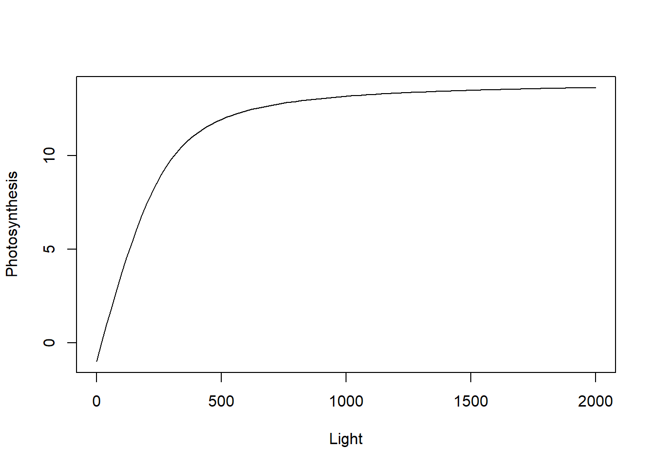
The parameter Rd stands for respiration and is assumed to be independent of light, so it is a value that shifts the curve downwards. The parameter alpha is the initial slope of the curve at low light intensity (denoted quantum yield of photosynthesis), Pmax is the asymptoptic maximum value of photosynthesis (i.e., the plateau at high light) and theta is a parameter that controls how fast the curve reaches that plateau.
11.3.1 Non-linear model
We start with a single curve that we will fit with brms.
photosynthesis <- read.csv("data/raw/PhotosynthesisArabidopsisRaw.csv")[1:9,]
with(photosynthesis, plot(P~I))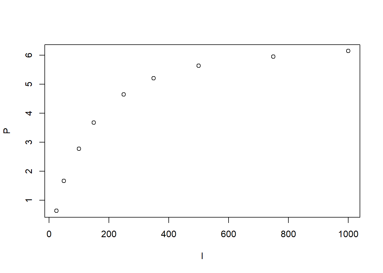
The parameters in the model are all constrained so the default WIP will not work. Scaling the prediction does not work either (since the relationship between I and P is non-linear). Furthermore, photosynthesis in an area where we do have a lot of prior knowledge (these parameters have been estimated thousands of times before). So here I will use informative priors.
Let’s first check what are the names that brms assigns to the parameters in the model. First we create a non-linear formula in brms using bf() with nl = TRUE. Note that in brms you need to specify an additional linear formula for every parameter in a model. In the simplest case where we have a single replicate we just specify a single parameter value as lf(par~1) (later we will expand this to include fixed and random effects on the non-linear parameters):
model <- bf(P~(alpha*I + Pmax - sqrt((alpha*I + Pmax)^2 - 4*alpha*I*theta*Pmax))/(2*theta) - Rd,
            lf(alpha~1),
            lf(theta~1),
            lf(Pmax~1),
            lf(Rd~1),
            nl = TRUE)
model
P ~ (alpha * I + Pmax - sqrt((alpha * I + Pmax)^2 - 4 * alpha * I * theta * Pmax))/(2 * theta) - Rd
alpha ~ 1
theta ~ 1
Pmax ~ 1
Rd ~ 1We can now check the default priors
default_prior(model, data = photosynthesis) prior class coef group resp dpar nlpar lb ub source
student_t(3, 0, 2.5) sigma 0 default
(flat) b alpha default
(flat) b Intercept alpha (vectorized)
(flat) b Pmax default
(flat) b Intercept Pmax (vectorized)
(flat) b Rd default
(flat) b Intercept Rd (vectorized)
(flat) b theta default
(flat) b Intercept theta (vectorized)As always we see quite some redundancy in this output, but the idea is that we have four intercept parameters (one per non-linear parameter) plus the standard deviation of observations sigma. I will create some informative priors (as an expert on the topic) also including biological constraints on the parameters. For simplicity I use constrained normal distributions:
priors <- prior("normal(0.05, 0.03)", class = "b",  nlpar = "alpha", lb = 0.0, ub = 0.125) +
          prior("normal(0.7, 0.3)", class = "b",  nlpar = "theta", lb = 0.0, ub = 1.0) +
          prior("normal(1, 1)", class = "b",  nlpar = "Rd", lb = 0.0) +
          prior("normal(15, 10)", class = "b",  nlpar = "Pmax", lb = 0.0) +
          prior("normal(0, 2)", class = "sigma", lb = 0.0)
We are now ready to fit the model:
if(RUN) {
    fit_photo1 <- brm(model, data = photosynthesis, prior = priors, seed = 123,
                    backend = "cmdstanr", save_model = "stan/photo_1",
                    control = list(adapt_delta = 0.99), iter = 4000, warmup = 1000)
} else {
    fit_photo1 <- readRDS("data/processed/photo_1.rds")
}
#saveRDS(fit_photo1, "data/processed/photo_1.rds")
summary(fit_photo1)
Family: gaussian
Links: mu = identity; sigma = identity
Formula: P ~ (alpha * I + Pmax - sqrt((alpha * I + Pmax)^2 - 4 * alpha * I * theta * Pmax))/(2 * theta) - Rd
alpha ~ 1
theta ~ 1
Pmax ~ 1
Rd ~ 1
Data: photosynthesis (Number of observations: 9)
Draws: 4 chains, each with iter = 4000; warmup = 1000; thin = 1;
total post-warmup draws = 12000
Regression Coefficients:
Estimate Est.Error l-95% CI u-95% CI Rhat Bulk_ESS Tail_ESS
alpha_Intercept 0.05 0.01 0.04 0.07 1.00 2082 2722
theta_Intercept 0.40 0.14 0.11 0.64 1.00 2387 2643
Pmax_Intercept 7.21 0.27 6.70 7.74 1.00 2192 2871
Rd_Intercept 0.46 0.20 0.11 0.88 1.00 2075 1939
Further Distributional Parameters:
Estimate Est.Error l-95% CI u-95% CI Rhat Bulk_ESS Tail_ESS
sigma 0.08 0.04 0.04 0.18 1.00 2261 3152
Draws were sampled using sample(hmc). For each parameter, Bulk_ESS
and Tail_ESS are effective sample size measures, and Rhat is the potential
scale reduction factor on split chains (at convergence, Rhat = 1).Diagnostics look good (Rhat = 1.0 and effective sample sizes in the thousands, note that I did increase the number of iterations to 4000 from the default 2000 to get enough samples, non-linear models are tough to work with!).
We can compare the observations to the predictions of the model:
library(Hmisc)
predictions <- predict(fit_photo1)
head(predictions)
Estimate Est.Error Q2.5 Q97.5
[1,] 0.6679806 0.1194392 0.4196637 0.8990633
[2,] 1.5655689 0.1088195 1.3526087 1.7771658
[3,] 2.8523355 0.1072180 2.6405007 3.0663896
[4,] 3.6891601 0.1049225 3.4815796 3.9062982
[5,] 4.6514078 0.1038435 4.4449966 4.8681782
[6,] 5.1684590 0.1031718 4.9663869 5.3733861with(photosynthesis, plot(P~I, cex = 2))
errbar(photosynthesis$I, predictions[,1], predictions[,4], predictions[,3],col = 2,
errbar.col = 2, add = TRUE)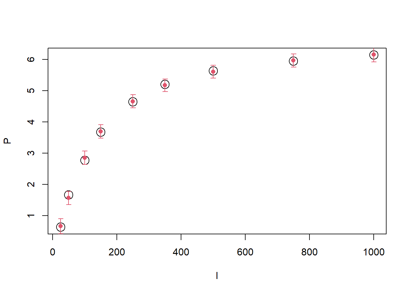
We can see that the model fits the data quite well (and any difference is well within the uncertainty of predictions). We can compare the prior and posterior distributions:
posterior <- as.data.frame(fit_photo1)
par(mfrow = c(2,2))
curve(dnorm(x, 0.05, 0.03), 0, 0.125, xlab = "alpha", ylim = c(0, 60))
lines(density(posterior$b_alpha_Intercept, from = 0, to = 0.125), col = 2)
curve(dnorm(x, 0.7, 0.3), 0, 1, xlab = "theta", ylim = c(0, 3))
lines(density(posterior$b_theta_Intercept, from = 0, to = 1), col = 2)
curve(dnorm(x, 15, 5), 0, 20, xlab = "Pmax", ylim = c(0,1.5))
lines(density(posterior$b_Pmax_Intercept, from = 0), col = 2)
curve(dnorm(x, 1, 1), 0, 3, xlab = "Rd", ylim = c(0,3))
lines(density(posterior$b_Rd_Intercept, from = 0), col = 2)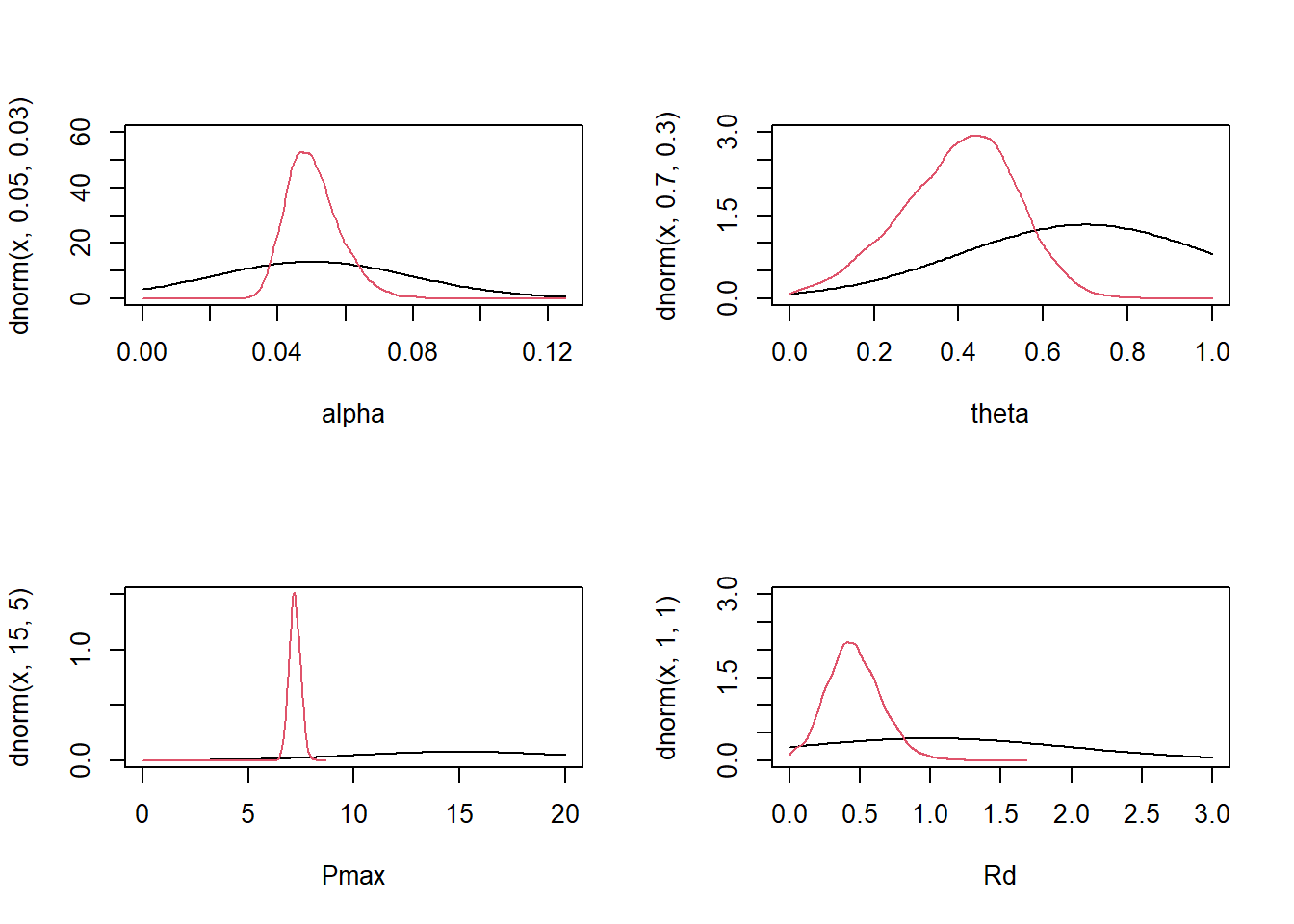
par(mfrow = c(1,1))We were able to learn quite a bit of information for each parameter, even when the posterior seems to disagree with our prior estimates (because our priors were not too informative, the data still dominates the posterior).
11.3.2 Non-linear models with random effect on parameters
Let’s extend the model to include random effects on the parameters (measuring the variation across individuals). Below I select all the measurements done on the reference or control level of the experiment:
photosynthesis <- subset(read.csv("data/raw/PhotosynthesisArabidopsisRaw.csv"), T == "LT" & W == "C")
with(photosynthesis, plot(P~I, col = Replicate))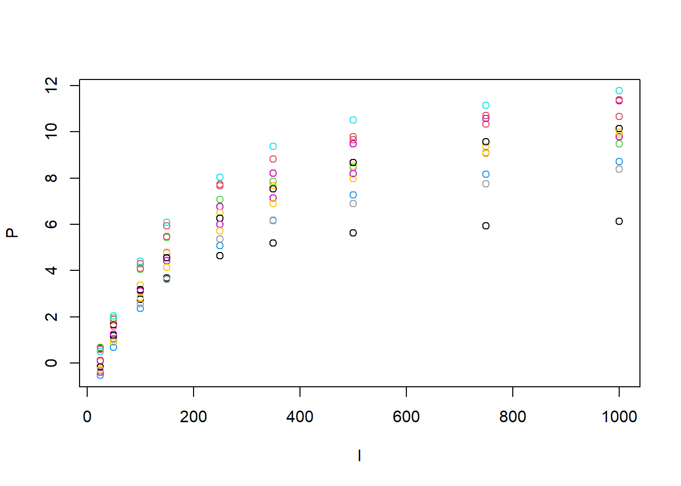
From the plot we can guess that both Pmax and Rd are going to vary across individuals but maybe also theta and alpha. It is also clear that at least Pmax and Rd are correlated across individuals (curves with lower Pmax would also have lower Rd). However, we will first ignore this and assume that each trait is independent. The formula of the model now looks like this:
model_rep <- bf(P~(alpha*I + Pmax - sqrt((alpha*I + Pmax)^2 - 4*alpha*I*theta*Pmax))/(2*theta) - Rd,
            # Transform parameters (link functions that also ensure proper scaling)
            nlf(Pmax  ~ exp(uPmax)), # Forces Pmax > 0
            nlf(theta ~ 1/(1 + exp(-utheta))), # Forces 0 < theta < 1
            nlf(alpha ~ 1/(1 + exp(-ualpha))*0.125), # Forces 0 < alpha < 0.125
            nlf(Rd    ~ exp(uRd)), # Forces Rd > 0
            lf(ualpha~1 + (1 | Replicate)),
            lf(utheta~1 + (1 | Replicate)),
            lf(uPmax~1 + (1 | Replicate)),
            lf(uRd~1 + (1 | Replicate)),
            nl = TRUE)
model_rep
P ~ (alpha * I + Pmax - sqrt((alpha * I + Pmax)^2 - 4 * alpha * I * theta * Pmax))/(2 * theta) - Rd
Pmax ~ exp(uPmax)
theta ~ 1/(1 + exp(-utheta))
alpha ~ 1/(1 + exp(-ualpha)) * 0.125
Rd ~ exp(uRd)
ualpha ~ 1 + (1 | Replicate)
utheta ~ 1 + (1 | Replicate)
uPmax ~ 1 + (1 | Replicate)
uRd ~ 1 + (1 | Replicate)That looks a lot more complex. The issue is that we can only use linear mixed models on the parameters of the non-linear model (strictly speaking because of a limitation in brms, but also because glmm on parameters of non-linear models are very difficult to fit). Since the parameters are constrained, we cannot model them directly with a linear mixed model, instead we need to transform them into unconstrained variables (e.g., uPmax is the log of Pmax and uRd is the log of Rd). This is analogous to the link functions that we used in generalized linear models (as the means of those models are also constrained). These transformations are the ones in the nlf() formulae and will complicate the rest of the analysis. Just to be clear, this is not a limitation of Bayesian inference but of this type of non-linear models.
We need to specify the priors for the mean and standard deviation on the random effects but this is tricky since we are now dealing with unconstrained variables. The best way is to just use simulation to figure out (approximately) what the prior on the mean values of the parameters should be (i.e., generate a large sample from the original prior, transform and check the new mean and standard deviation):
library(truncnorm)
# Prior expectation for mean and sd of uPmax
Pmaxs <- rtruncnorm(1e6, 15, 5, a = 0)
uPmaxs <- log(Pmaxs)
mean_uPmax <- mean(uPmaxs)
sd_uPmax <- sd(uPmaxs)
c(mean_uPmax, sd_uPmax)
[1] 1.5878295 0.2119576# Prior expectation for mean and sd of uRd
Rds <- rtruncnorm(1e6, 1, 1, a = 0)
uRds <- log(Rds)
mean_uRd <- mean(uRds)
sd_uRd <- sd(uRds)
c(mean_uRd, sd_uRd)[1] -1.000497 1.000209# Prior expectation for mean and sd of ualpha
alphas <- rtruncnorm(1e6, 0.05, 0.03, a = 0, b = 0.125)
ualphas <- log(alphas/(0.125 - alphas))
mean_ualpha <- mean(ualphas)
sd_ualpha <- sd(ualphas)
c(mean_ualpha, sd_ualpha)[1] -0.4144967 1.1716053# Prior expectation for mean and sd of utheta
thetas <- rtruncnorm(1e6, 0.7, 0.3, a = 0, b = 1)
uthetas <- log(thetas/(1 - thetas))
mean_utheta <- mean(uthetas)
sd_utheta <- sd(uthetas)
c(mean_utheta, sd_utheta)[1] 0.676853 1.359461Of course you could also try to calculate this mean and standard deviation analytically (be my guest) but please do not just apply the transformation to the mean and standard deviation of the original prior, that will not be correct (i.e., if the mean of Pmax is 15, the mean of uPmax = log(Pmax) is not log(15)!).
These values may be used to build the prior distributions on the means of the uconstrained parameters (i.e., the Intercept coefficients in the linear mixed models associated to non-linear parameters). What about the variation across replicates? This is a bit more tricky to assess from literature since the focus of research is always on mean effects rather than variation and the actual variation also depends very much on the experiment (i.e., a good experiment will have less variation across individuals that are genetically identical and are grown under the same environmental conditions). Of course, if we have access to the raw data of similar experiments we could get a good estimate.
Alternatively we can try to calculate this variation relative to the mean (e.g., we expect the standard deviation across replicates to be 30% of the mean) but also add a significant level of uncertainty to this prior since it is just a rough estimate (e.g., 50%).
Let’s build the priors using these rules. First we extract the default priors to know which names brms is using:
default_prior(model_rep, data = photosynthesis) prior class coef group resp dpar nlpar lb ub
student_t(3, 0, 4.2) sigma 0
(flat) b ualpha
(flat) b Intercept ualpha
student_t(3, 0, 4.2) sd ualpha 0
student_t(3, 0, 4.2) sd Replicate ualpha 0
student_t(3, 0, 4.2) sd Intercept Replicate ualpha 0
(flat) b uPmax
(flat) b Intercept uPmax
student_t(3, 0, 4.2) sd uPmax 0
student_t(3, 0, 4.2) sd Replicate uPmax 0
student_t(3, 0, 4.2) sd Intercept Replicate uPmax 0
(flat) b uRd
(flat) b Intercept uRd
student_t(3, 0, 4.2) sd uRd 0
student_t(3, 0, 4.2) sd Replicate uRd 0
student_t(3, 0, 4.2) sd Intercept Replicate uRd 0
(flat) b utheta
(flat) b Intercept utheta
student_t(3, 0, 4.2) sd utheta 0
student_t(3, 0, 4.2) sd Replicate utheta 0
student_t(3, 0, 4.2) sd Intercept Replicate utheta 0
source
default
default
(vectorized)
default
(vectorized)
(vectorized)
default
(vectorized)
default
(vectorized)
(vectorized)
default
(vectorized)
default
(vectorized)
(vectorized)
default
(vectorized)
default
(vectorized)
(vectorized)For each unconstrain parameter we need to define to priors (Intercept and sd under Replicate):
priors <- prior("normal(-0.4, 1.17)", class = "b",  coef = "Intercept", nlpar = "ualpha") +
          prior("normal(0.12, 0.06)", class = "sd", group = "Replicate", nlpar = "ualpha", lb = 0) +
          prior("normal(0.67, 1.35", class = "b",  coef = "Intercept", nlpar = "utheta") +
          prior("normal(0.20, 0.1)", class = "sd", group = "Replicate", nlpar = "utheta", lb = 0) +
          prior("normal(-1.0, 1.0)", class = "b",  coef = "Intercept", nlpar = "uRd") +
          prior("normal(0.3, 0.15)", class = "sd", group = "Replicate", nlpar = "uRd", lb = 0) +
          prior("normal(1.6, 0.21)", class = "b",  coef = "Intercept", nlpar = "uPmax") +
          prior("normal(0.48, 0.24)", class = "sd", group = "Replicate", nlpar = "uPmax", lb = 0) +
          prior("normal(0, 2)", class = "sigma", lb = 0.0)
priors
prior class coef group resp dpar nlpar lb ub source
normal(-0.4, 1.17) b Intercept ualpha <NA> <NA> user
normal(0.12, 0.06) sd Replicate ualpha 0 <NA> user
normal(0.67, 1.35 b Intercept utheta <NA> <NA> user
normal(0.20, 0.1) sd Replicate utheta 0 <NA> user
normal(-1.0, 1.0) b Intercept uRd <NA> <NA> user
normal(0.3, 0.15) sd Replicate uRd 0 <NA> user
normal(1.6, 0.21) b Intercept uPmax <NA> <NA> user
normal(0.48, 0.24) sd Replicate uPmax 0 <NA> user
normal(0, 2) sigma 0 <NA> userWe are now ready to fit the model:
if(RUN) {
    fit_photo2 <- brm(model_rep, data = photosynthesis, prior = priors, seed = 123,
                    backend = "cmdstanr", save_model = "stan/photo_2",
                    control = list(adapt_delta = 0.99, max_treedepth = 15), iter = 4000, warmup = 1000)
} else {
    fit_photo2 <- readRDS("data/processed/fit_photo2.rds")
}
summary(fit_photo2)
Family: gaussian
Links: mu = identity; sigma = identity
Formula: P ~ (alpha * I + Pmax - sqrt((alpha * I + Pmax)^2 - 4 * alpha * I * theta * Pmax))/(2 * theta) - Rd
Pmax ~ exp(uPmax)
theta ~ 1/(1 + exp(-utheta))
alpha ~ 1/(1 + exp(-ualpha)) * 0.125
Rd ~ exp(uRd)
ualpha ~ 1 + (1 | Replicate)
utheta ~ 1 + (1 | Replicate)
uPmax ~ 1 + (1 | Replicate)
uRd ~ 1 + (1 | Replicate)
Data: photosynthesis (Number of observations: 108)
Draws: 4 chains, each with iter = 4000; warmup = 1000; thin = 1;
total post-warmup draws = 12000
Multilevel Hyperparameters:
~Replicate (Number of levels: 12)
Estimate Est.Error l-95% CI u-95% CI Rhat Bulk_ESS
sd(ualpha_Intercept) 0.20 0.04 0.12 0.29 1.00 8410
sd(utheta_Intercept) 0.43 0.09 0.26 0.60 1.00 7294
sd(uPmax_Intercept) 0.25 0.09 0.14 0.48 1.00 3132
sd(uRd_Intercept) 0.28 0.07 0.16 0.44 1.00 6418
Tail_ESS
sd(ualpha_Intercept) 8316
sd(utheta_Intercept) 6095
sd(uPmax_Intercept) 5122
sd(uRd_Intercept) 6992
Regression Coefficients:
Estimate Est.Error l-95% CI u-95% CI Rhat Bulk_ESS Tail_ESS
ualpha_Intercept 0.11 0.09 -0.06 0.30 1.00 8535 7729
utheta_Intercept -0.83 0.22 -1.28 -0.42 1.00 10145 8687
uPmax_Intercept 2.42 0.09 2.19 2.57 1.00 2466 3961
uRd_Intercept 0.27 0.10 0.07 0.46 1.00 4874 6550
Further Distributional Parameters:
Estimate Est.Error l-95% CI u-95% CI Rhat Bulk_ESS Tail_ESS
sigma 0.10 0.01 0.08 0.12 1.00 6129 7628
Draws were sampled using sample(hmc). For each parameter, Bulk_ESS
and Tail_ESS are effective sample size measures, and Rhat is the potential
scale reduction factor on split chains (at convergence, Rhat = 1).#saveRDS(fit_photo2, "data/processed/fit_photo2.rds")This took longer than previous model runs. This is a consequence of the larger number of parameters (fixed and random effects) and the more complex shape of the distribution (due the non-linear transformations in the model). Diagnostics (Rhat and effective sample sizes) look fine. The effective sample sizes are large enough.
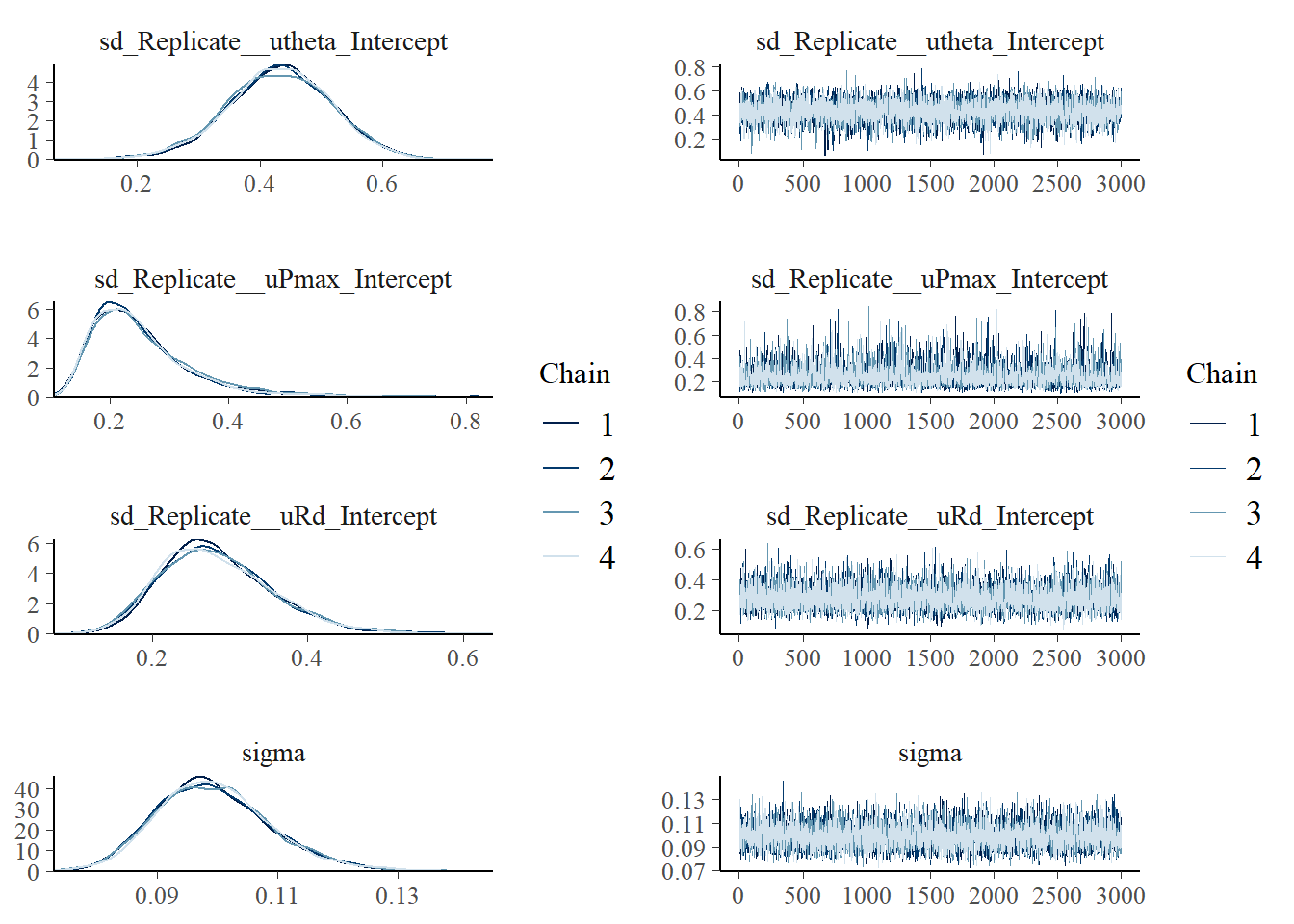
We can double check the traces of the chains and the posteriors generated by each chain:
plot(fit_photo2, combo = c("dens_overlay", "trace"))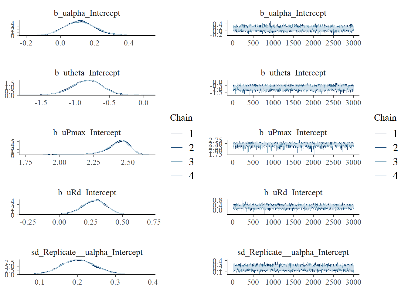
Checking the fit to observations is a bit more complex since we have multiple curves. We can always plot observed vs predicted values (with uncertainty!).
library(posterior)
posterior <- subset_draws(as_draws_df(fit_photo2), iteration = seq(1, 3000, by = 2)) # thin = 2
predictions <- as.data.frame(predict(fit_photo2))
photosynthesis$Ppred <- predictions$Estimate
photosynthesis$PpredQ2.5 <- predictions$Q2.5
photosynthesis$PpredQ97.5 <- predictions$Q97.5
with(photosynthesis, errbar(P, Ppred, PpredQ97.5, PpredQ2.5, col = Replicate, errbar.col = Replicate))
abline(a = 0, b = 1, lty = 2)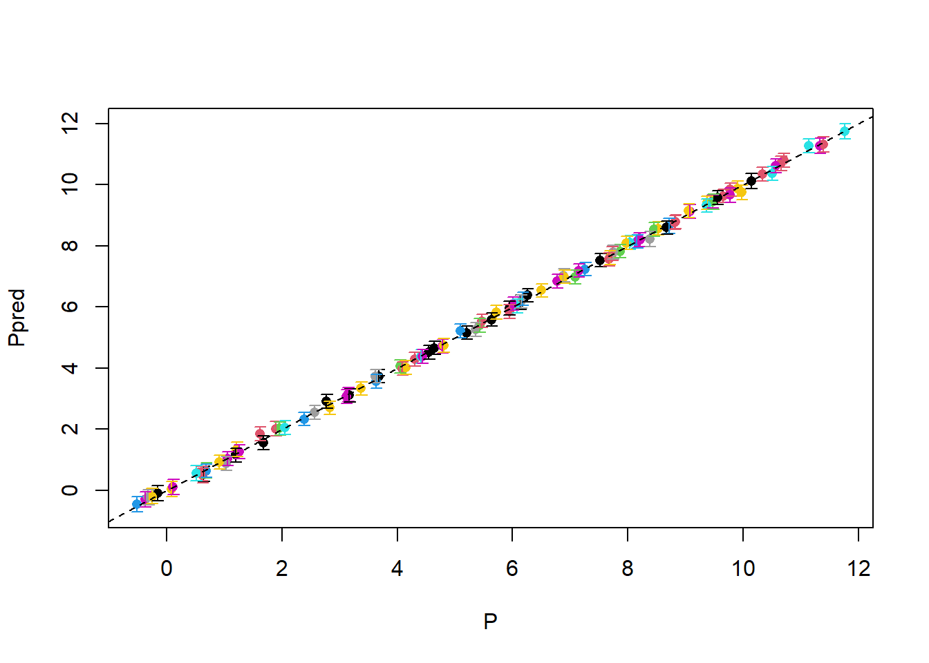
This is essentially a perfect fit!
Ok, now let’s interpret the results. Because of the non-linear transformations it is a bit difficult to interpret the meaning of the intercepts and random effects (i.e., I have a good feeling what a typical Pmax value is, but log(uPmax)?). This means that to interpret the results we need to transform the estimates back to the original scale. As before, we should not take the mean of the posterior and transform it back (that will give the wrong result) but rather we should transform the entire sample of posterior draws and then calculate the means, quantiles, etc.
The presence of a hierarchical structure makes a bit more complex but, as we have a distribution of distributions. The idea is that each sample of the posterior defines a different distribution of the parameters across individuals (i.e., each value of b_ualpha_Intercept and sd_Replicate__ualpha_Intercept defines a distribution of ualpha across replicates). So here we can choose multiple possible approaches:
Estimate the values of the parameters in the original scale for individual groups (i.e, e.g., the values of
alphathat the model estimates for each leaf that was measured).Estimate the mean and standard deviation in the original scale for each parameter (like we did for the priors but in reverse). That is,
sd_Replicate__alpha_Interceptandb_alpha_Intercept(notice that I removed theuprefix).Generate a sample from the distribution of parameter values across replicates (i.e., the distribution of individual
alphavalues).
11.3.2.1 Back transformation of individual estimates
Fortunately we can achieve this with the fitted() function in brms that if we specify the right non-linear parmaeter. Note that this will return the estimate for each measurement point (but every nine data points correspond to the same leaf, so we have each estimate repeated nine times, we can avoid this by using the unique() function):
alphas <- unique(fitted(fit_photo2, nlpar = "alpha"))
thetas <- unique(fitted(fit_photo2, nlpar = "theta"))
Pmaxs <- unique(fitted(fit_photo2, nlpar = "Pmax"))
Rds <- unique(fitted(fit_photo2, nlpar = "Rd"))
Note that most of the time we are not interested in the estiamtes for each individual but on the population level estimates, but this can be useful when dealing with outliers or extreme values.
Let’s visualize the mean estimates for all parameters and replicates:
pairs(cbind(alpha = alphas[,1], theta = thetas[,1], Pmax = Pmaxs[,1], Rd = Rds[,1]))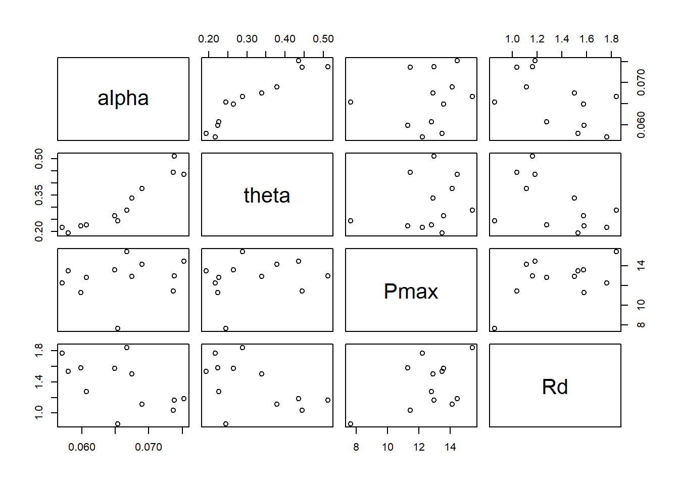
As expected from the visualization, the parameters are correlated across individuals, even if our model does not try to assume that correlation.
11.3.2.2 Back transformation of fixed and random effects
If I want to estimate sd_Replicate__alpha_Intercept and b_alpha_Intercept from sd_Replicate__ualpha_Intercept and b_ualpha_Intercept I need to follow two nested steps (or only one if I know how backtransform analytically, but I show you the more general approach):
- For each sample of the posterior, generate a large samples of
ualphavalues - Backtransform the distributtion of
ualphavalues to the original scale and calculate the mean and standard deviation of that distribution.
Let’s do this:
sd_Replicate__alpha_Intercept <- numeric(length(posterior$sd_Replicate__ualpha_Intercept))
b_alpha_Intercept <- numeric(length(posterior$b_ualpha_Intercept))
for(i in 1:nrow(posterior)) {
    # Sample from the distribution of ualpha
    ualphas <- rnorm(1e3, posterior$b_ualpha_Intercept[i], posterior$sd_Replicate__ualpha_Intercept[i])
    # Backtransform to alpha
    alphas <- 1/(1 + exp(-ualphas))*0.125
    # Calculate mean and sd of alpha
    sd_Replicate__alpha_Intercept[i] <- sd(alphas)
    b_alpha_Intercept[i] <- mean(alphas)
}
summary(sd_Replicate__alpha_Intercept)
Min. 1st Qu. Median Mean 3rd Qu. Max.
0.001540 0.005317 0.006201 0.006232 0.007113 0.012603 plot(density(sd_Replicate__alpha_Intercept))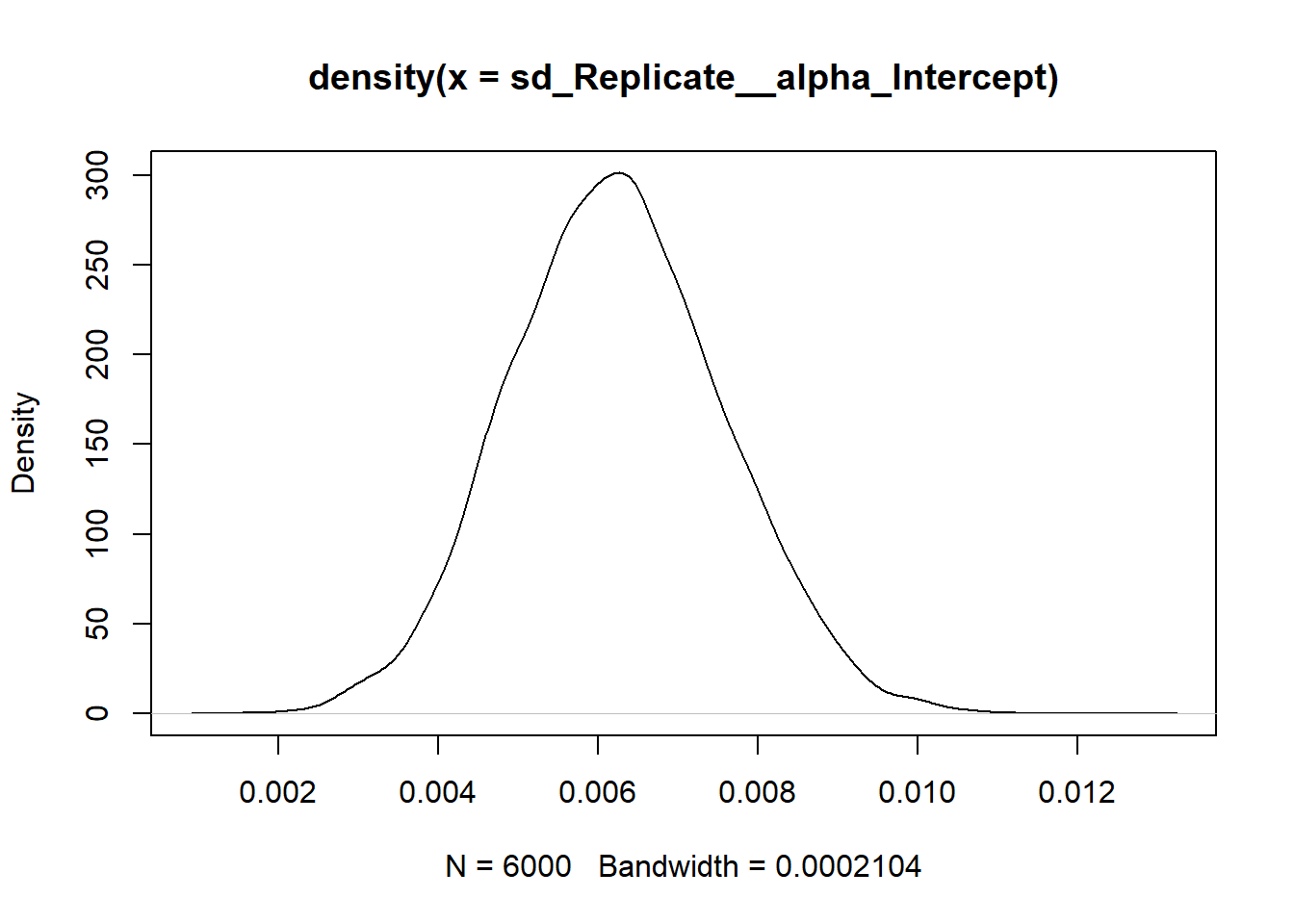
summary(b_alpha_Intercept) Min. 1st Qu. Median Mean 3rd Qu. Max.
0.05519 0.06413 0.06593 0.06597 0.06774 0.07922 plot(density(b_alpha_Intercept))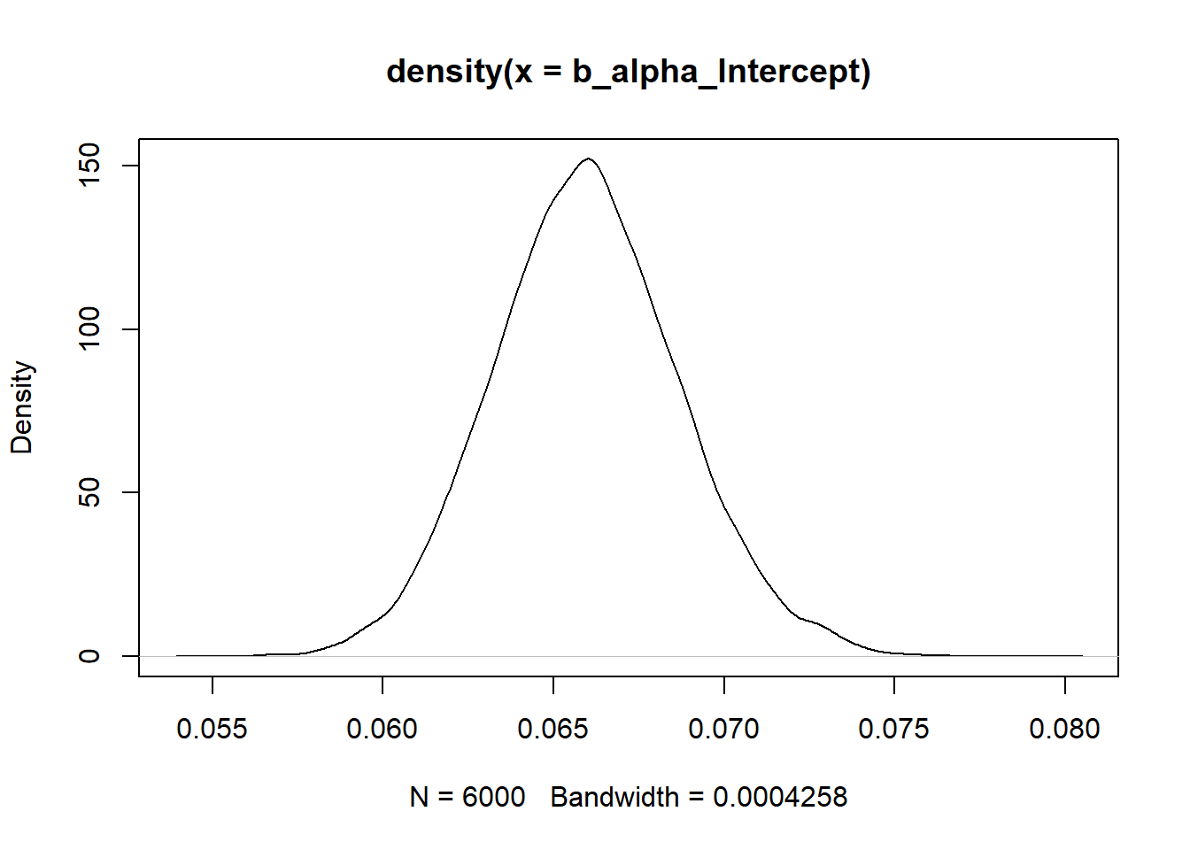
11.3.2.3 Predictions of new individuals
In the previous section we estimated the mean and standard deviation of alpha across replicates or the best estimates of alpha for the leaves that were onbserved. However, we can also generate a sample of individual alpha values that combine both variation and uncertainty. This distributions is our prediction for a new leaf that we could measure from the same population.
I find this distribution useful for understanding what the random effects actually imply and because statistical inference is about generalizing to new individuals and not just about the individuals that were observed (i.e., the replicates).
This is actually easier to achieve than the previous step. In this case we just need to generate a single sample from the distribution of ualpha, utheta, uPmax and uRd and then backtransform those values to the original scale. This would yield a prediction of parameter values that accounts for variation across replicates (i.e., the random effect) and the uncertainty we have about the parameters that govern that variation:
par(mfrow = c(2,2))
# Variation in alpha across individuals
ualphas <- rnorm(6e3, posterior$b_ualpha_Intercept, posterior$sd_Replicate__ualpha_Intercept)
alphas <- 1/(1 + exp(-ualphas))*0.125
plot(density(alphas))
abline(v = c(median(alphas), mean(alphas)), col = 2:3)
# Variation in theta across individuals
uthetas <- rnorm(6e3, posterior$b_utheta_Intercept, posterior$sd_Replicate__utheta_Intercept)
thetas <- 1/(1 + exp(-uthetas))
plot(density(thetas))
abline(v = c(median(thetas), mean(thetas)), col = 2:3)
# Variation in Pmax across individuals
uPmaxs <- rnorm(6e3, posterior$b_uPmax_Intercept, posterior$sd_Replicate__uPmax_Intercept)
Pmaxs <- exp(uPmaxs)
plot(density(Pmaxs))
abline(v = c(median(Pmaxs), mean(Pmaxs)), col = 2:3)
# Variation in Rd across individuals
uRds <- rnorm(6e3, posterior$b_uRd_Intercept, posterior$sd_Replicate__uRd_Intercept)
Rds <- exp(uRds)
plot(density(Rds))
abline(v = c(median(Rds), mean(Rds)), col = 2:3)
par(mfrow = c(1,1))We can plot the variation in all parameters across individuals but we should not expect any correlation because these are predictions from the model of a new individual:
pairs(cbind(alphas, thetas, Pmaxs, Rds))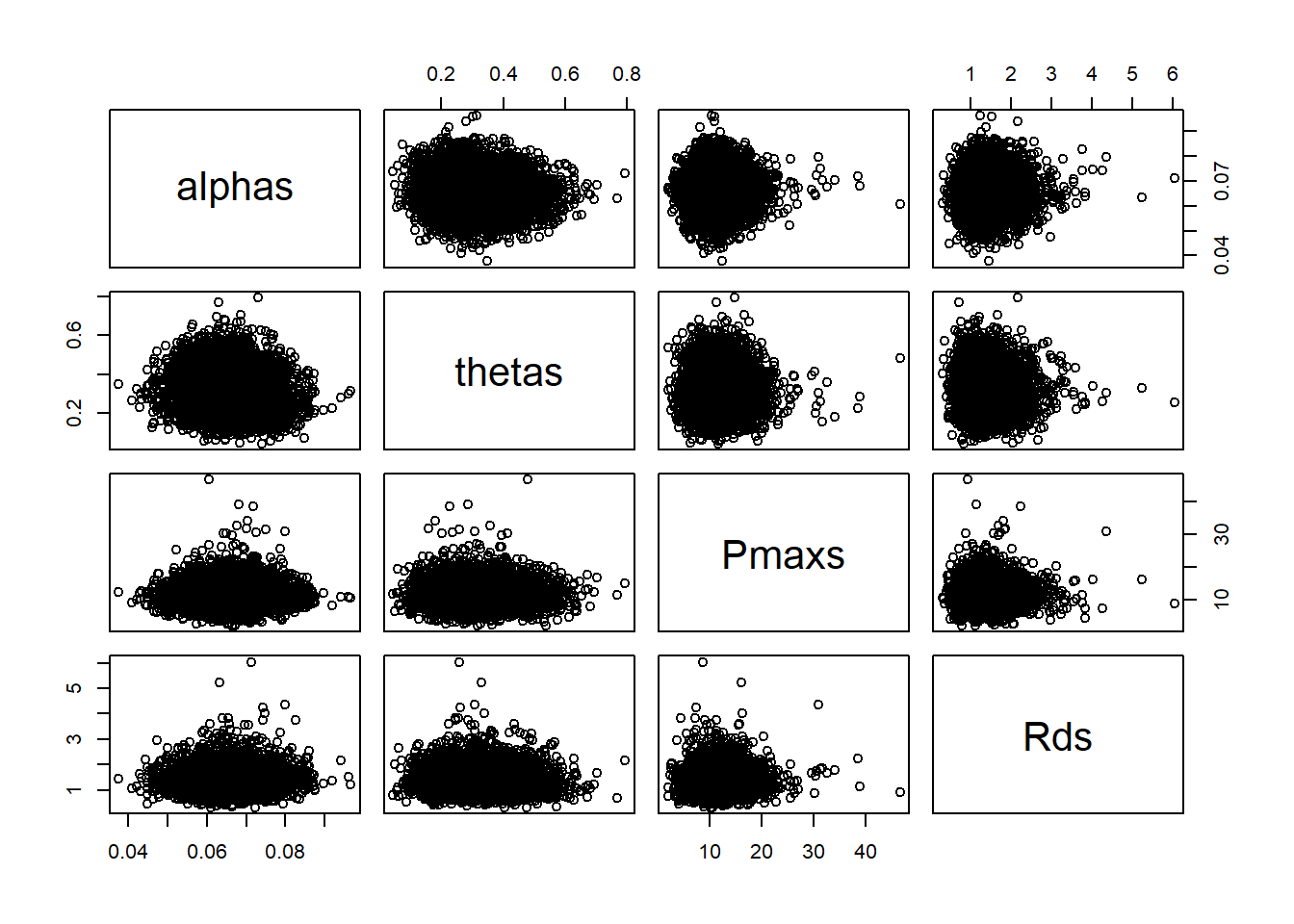
Comparing this pairs plot with the one we generated before (for the estimates of the actual leaves that were measured) is a strong hint that would should account for correlations among these parameters in the model.
11.3.3 Non-linear models with correlated random effects on parameters
Let’s now take into account the fact that traits are correlated across individiuals. This can be achieved by adding a label to random effects component of the linear mixed model assign to each parameter. The label is placed between | inside the random effect:
model_rep_cor <- bf(
            P~(alpha*I + Pmax - sqrt((alpha*I + Pmax)^2 - 4*alpha*I*theta*Pmax))/(2*theta) - Rd,
            # Transform parameters (link functions that also ensure proper scaling)
            nlf(Pmax  ~ exp(uPmax)), # Forces Pmax > 0
            nlf(theta ~ 1/(1 + exp(-utheta))), # Forces 0 < theta < 1
            nlf(alpha ~ 1/(1 + exp(-ualpha))*0.125), # Forces 0 < alpha < 0.125
            nlf(Rd    ~ exp(uRd)), # Forces Rd > 0
            ualpha~1 + (1 | leaf_trait | Replicate),
            utheta~1 + (1 | leaf_trait | Replicate),
            uPmax~1 + (1 | leaf_trait | Replicate),
            uRd~1 + (1 | leaf_trait | Replicate),
            nl = TRUE)
default_prior(model_rep_cor, data = photosynthesis)
prior class coef group resp dpar nlpar lb ub
lkj(1) cor
lkj(1) cor Replicate
student_t(3, 0, 4.2) sigma 0
(flat) b ualpha
(flat) b Intercept ualpha
student_t(3, 0, 4.2) sd ualpha 0
student_t(3, 0, 4.2) sd Replicate ualpha 0
student_t(3, 0, 4.2) sd Intercept Replicate ualpha 0
(flat) b uPmax
(flat) b Intercept uPmax
student_t(3, 0, 4.2) sd uPmax 0
student_t(3, 0, 4.2) sd Replicate uPmax 0
student_t(3, 0, 4.2) sd Intercept Replicate uPmax 0
(flat) b uRd
(flat) b Intercept uRd
student_t(3, 0, 4.2) sd uRd 0
student_t(3, 0, 4.2) sd Replicate uRd 0
student_t(3, 0, 4.2) sd Intercept Replicate uRd 0
(flat) b utheta
(flat) b Intercept utheta
student_t(3, 0, 4.2) sd utheta 0
student_t(3, 0, 4.2) sd Replicate utheta 0
student_t(3, 0, 4.2) sd Intercept Replicate utheta 0
source
default
(vectorized)
default
default
(vectorized)
default
(vectorized)
(vectorized)
default
(vectorized)
default
(vectorized)
(vectorized)
default
(vectorized)
default
(vectorized)
(vectorized)
default
(vectorized)
default
(vectorized)
(vectorized)Here, ualpha, utheta, uPmax and uRd are assumed to be correlated across replicates because they all have the label leaf_trait. This will introduce an additional prior, the LKJ prior on the correlation matrix that we saw before. We can assign an WIP LKJ(2) as before:
priors <- prior("normal(-0.4, 1.17)", class = "b",  coef = "Intercept", nlpar = "ualpha") +
          prior("normal(0.12, 0.06)", class = "sd", group = "Replicate", nlpar = "ualpha", lb = 0) +
          prior("normal(0.67, 1.35", class = "b",  coef = "Intercept", nlpar = "utheta") +
          prior("normal(0.20, 0.1)", class = "sd", group = "Replicate", nlpar = "utheta", lb = 0) +
          prior("normal(-1.0, 1.0)", class = "b",  coef = "Intercept", nlpar = "uRd") +
          prior("normal(0.3, 0.15)", class = "sd", group = "Replicate", nlpar = "uRd", lb = 0) +
          prior("normal(1.6, 0.21)", class = "b",  coef = "Intercept", nlpar = "uPmax") +
          prior("normal(0.48, 0.24)", class = "sd", group = "Replicate", nlpar = "uPmax", lb = 0) +
          prior("normal(0, 2)", class = "sigma", lb = 0.0) +
          prior("lkj(2)", class = "cor")
priors
prior class coef group resp dpar nlpar lb ub source
normal(-0.4, 1.17) b Intercept ualpha <NA> <NA> user
normal(0.12, 0.06) sd Replicate ualpha 0 <NA> user
normal(0.67, 1.35 b Intercept utheta <NA> <NA> user
normal(0.20, 0.1) sd Replicate utheta 0 <NA> user
normal(-1.0, 1.0) b Intercept uRd <NA> <NA> user
normal(0.3, 0.15) sd Replicate uRd 0 <NA> user
normal(1.6, 0.21) b Intercept uPmax <NA> <NA> user
normal(0.48, 0.24) sd Replicate uPmax 0 <NA> user
normal(0, 2) sigma 0 <NA> user
lkj(2) cor <NA> <NA> userLet’s fit the model:
if(RUN) {
    fit_photo3 <- brm(model_rep_cor, data = photosynthesis, prior = priors, seed = 123,
                    backend = "cmdstanr", save_model = "stan/photo_3",
                    control = list(adapt_delta = 0.99, max_treedepth = 15), iter = 4000, warmup = 1000)
} else {
    fit_photo3 <- readRDS("data/processed/fit_photo3.rds")
}
summary(fit_photo3)
Family: gaussian
Links: mu = identity; sigma = identity
Formula: P ~ (alpha * I + Pmax - sqrt((alpha * I + Pmax)^2 - 4 * alpha * I * theta * Pmax))/(2 * theta) - Rd
Pmax ~ exp(uPmax)
theta ~ 1/(1 + exp(-utheta))
alpha ~ 1/(1 + exp(-ualpha)) * 0.125
Rd ~ exp(uRd)
ualpha ~ 1 + (1 | leaf_trait | Replicate)
utheta ~ 1 + (1 | leaf_trait | Replicate)
uPmax ~ 1 + (1 | leaf_trait | Replicate)
uRd ~ 1 + (1 | leaf_trait | Replicate)
Data: photosynthesis (Number of observations: 108)
Draws: 4 chains, each with iter = 4000; warmup = 1000; thin = 1;
total post-warmup draws = 12000
Multilevel Hyperparameters:
~Replicate (Number of levels: 12)
Estimate Est.Error l-95% CI u-95% CI
sd(ualpha_Intercept) 0.18 0.04 0.10 0.26
sd(utheta_Intercept) 0.43 0.08 0.27 0.58
sd(uPmax_Intercept) 0.23 0.07 0.14 0.41
sd(uRd_Intercept) 0.28 0.07 0.16 0.43
cor(ualpha_Intercept,utheta_Intercept) 0.55 0.21 0.09 0.89
cor(ualpha_Intercept,uPmax_Intercept) 0.17 0.28 -0.41 0.67
cor(utheta_Intercept,uPmax_Intercept) 0.08 0.23 -0.36 0.52
cor(ualpha_Intercept,uRd_Intercept) -0.11 0.29 -0.66 0.44
cor(utheta_Intercept,uRd_Intercept) -0.29 0.23 -0.69 0.20
cor(uPmax_Intercept,uRd_Intercept) 0.56 0.22 0.03 0.87
Rhat Bulk_ESS Tail_ESS
sd(ualpha_Intercept) 1.00 13059 7943
sd(utheta_Intercept) 1.00 11223 7454
sd(uPmax_Intercept) 1.00 4050 4500
sd(uRd_Intercept) 1.00 5135 7882
cor(ualpha_Intercept,utheta_Intercept) 1.00 8426 8528
cor(ualpha_Intercept,uPmax_Intercept) 1.00 2453 4719
cor(utheta_Intercept,uPmax_Intercept) 1.00 3506 5936
cor(ualpha_Intercept,uRd_Intercept) 1.00 2867 6295
cor(utheta_Intercept,uRd_Intercept) 1.00 4955 7473
cor(uPmax_Intercept,uRd_Intercept) 1.00 9914 7848
Regression Coefficients:
Estimate Est.Error l-95% CI u-95% CI Rhat Bulk_ESS Tail_ESS
ualpha_Intercept 0.10 0.09 -0.07 0.27 1.00 5914 7451
utheta_Intercept -0.85 0.22 -1.30 -0.43 1.00 9364 8289
uPmax_Intercept 2.44 0.08 2.24 2.56 1.00 4316 4579
uRd_Intercept 0.21 0.10 -0.01 0.39 1.00 6355 7202
Further Distributional Parameters:
Estimate Est.Error l-95% CI u-95% CI Rhat Bulk_ESS Tail_ESS
sigma 0.10 0.01 0.08 0.12 1.00 7593 8255
Draws were sampled using sample(hmc). For each parameter, Bulk_ESS
and Tail_ESS are effective sample size measures, and Rhat is the potential
scale reduction factor on split chains (at convergence, Rhat = 1).#saveRDS(fit_photo3, "data/processed/fit_photo3.rds")All looks good! Note that our estimates of correlations are quite uncertain and that is to be expected. Correlations are hard to estimate that variances and variances are harder to estimate than fixed effects. By harder I mean that, given a certain level of noise in the data, it takes more data to reduce uncertainty. For most combinations of parameters there does not seem to be a clear correlation except perhaps Rd vs Pmax (as expected) and alpha vs theta.
We want to reconstruct a population on individual traits in the original scale like we did before. We can follow the same approach as before but now we need to use a multivariate normal distribution.
First we extract the posterior distribution and thin the samples (based on the effective sample sizes we can take every other sample).
posterior <- subset_draws(as_draws_df(fit_photo3), iteration = seq(1, 3000, by = 2)) # thin = 2Then we construct a multivariate normal distribution that accounts for the correlations among the traits. This distribution takes as input a vector of means and a covariance matrix. The covariance can be reconstructed from the correlations and variances. Let’s do it for the first sample in the posterior distribution:
# Extract all the relevant variables form posterior (following brms naming system)
pars <- c("ualpha", "utheta", "uPmax", "uRd")
sds <- posterior[,paste0("sd_Replicate__",pars,"_Intercept")]
Warning: Dropping 'draws_df' class as required metadata was removed.rs <- posterior[,paste0("cor_Replicate__",pars[c(1,1,1,2,2,3)],"_Intercept__",pars[c(2,3,4,3,4,4)],"_Intercept")]Warning: Dropping 'draws_df' class as required metadata was removed.make_vcov <- function(i, sds, rs) {
# Extract sample from posterior
sd <- as.numeric(sds[i,])
r <- as.numeric(rs[i,])
# Construct correlation matrix
npar = length(sd)
Rho <- matrix(1, npar, npar)
Rho[upper.tri(Rho)] <- r
Rho[lower.tri(Rho)] <- t(Rho)[lower.tri(Rho)]
# Construct the variance covariance matrix
diag(sd) %*% Rho %*% diag(sd)
}
# Test the function
make_vcov(1, sds, rs) [,1] [,2] [,3] [,4]
[1,] 0.02348434 0.040300396 0.01667744 0.012911127
[2,] 0.04030040 0.216745182 -0.00975941 -0.008757671
[3,] 0.01667744 -0.009759410 0.03386262 0.026349910
[4,] 0.01291113 -0.008757671 0.02634991 0.070753340We can now generate samples from a multivariate normal distribution using mvtnorm:
library(mvtnorm)
mus <- posterior[,paste0("b_",pars,"_Intercept")]
sample_upars <- function(i, mus, sds, rs) {
    vcov <- make_vcov(i, sds, rs)
    mu   <- as.numeric(mus[i,])
    rmvnorm(1, mean = mu, sigma = vcov)
}
upars <- matrix(NA, nrow = nrow(posterior), ncol = 4)
for(i in 1:nrow(posterior)) {
    upars[i, ] <- sample_upars(i, mus, sds, rs)
}
# Let's add them back to the posterior data.frame
posterior$ualpha <- upars[,1]
posterior$utheta <- upars[,2]
posterior$uPmax <- upars[,3]
posterior$uRd <- upars[,4]
We are almost there! No we just need to backtransform them (we reuse the previous code)
par(mfrow = c(2,2))
# Variation in alpha across individuals
posterior$alpha <- 1/(1 + exp(-posterior$ualpha))*0.125
with(posterior, {
plot(density(alpha))
abline(v = c(median(alpha), mean(alpha)), col = 2:3)
})
# Variation in theta across individuals
posterior$theta <- 1/(1 + exp(-posterior$utheta))
with(posterior, {
plot(density(theta))
abline(v = c(median(theta), mean(theta)), col = 2:3)
})
# Variation in Pmax across individuals
posterior$Pmax <- exp(posterior$uPmax)
with(posterior, {
plot(density(Pmax))
abline(v = c(median(Pmax), mean(Pmax)), col = 2:3)
})
# Variation in Rd across individuals
posterior$Rd <- exp(posterior$uRd)
with(posterior, {
plot(density(Rd))
abline(v = c(median(Rd), mean(Rd)), col = 2:3)
})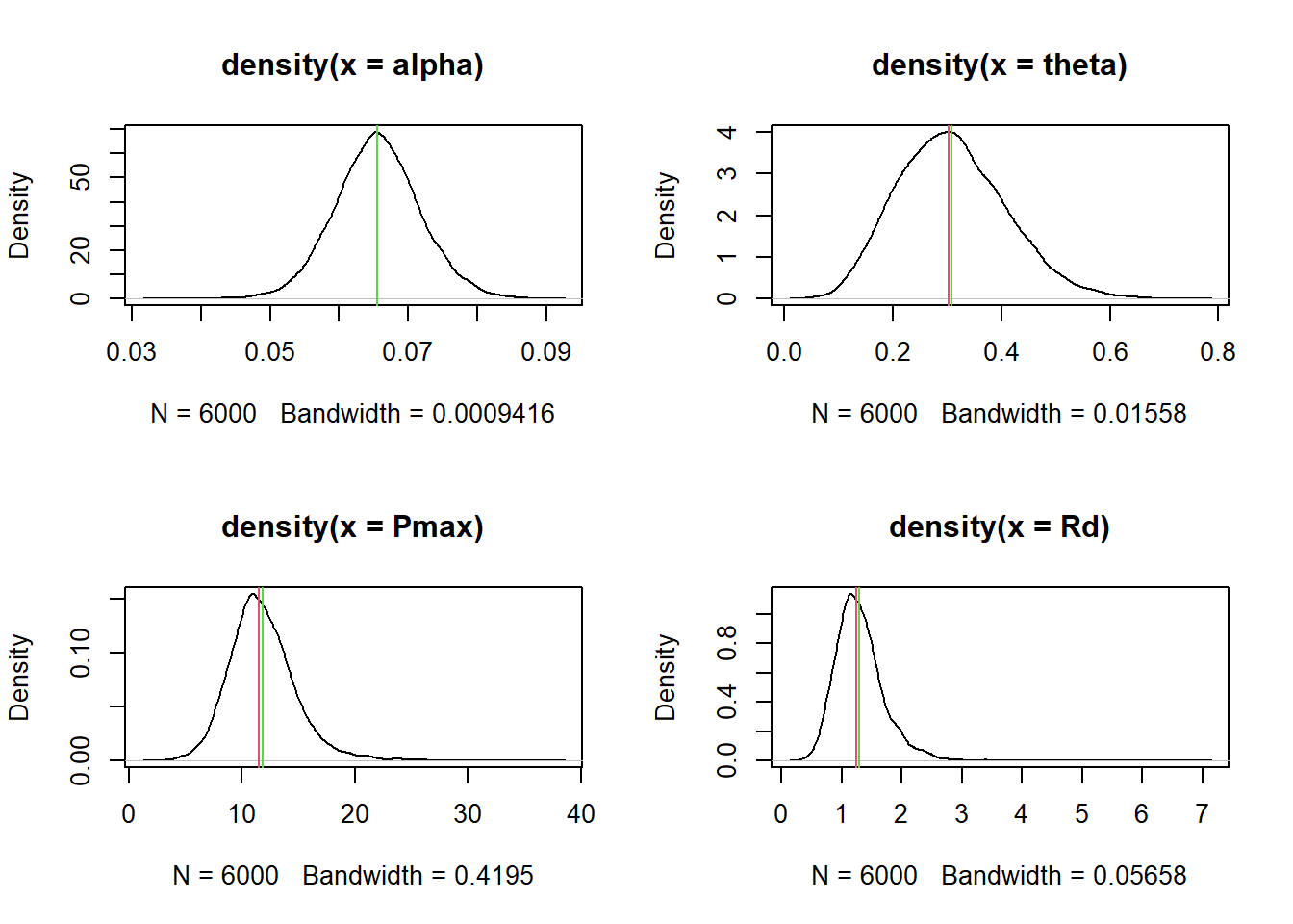
par(mfrow = c(1,1))But we can also see the correlations in the original scale:
pairs(posterior[,c("alpha", "theta", "Pmax", "Rd")])Warning: Dropping 'draws_df' class as required metadata was removed.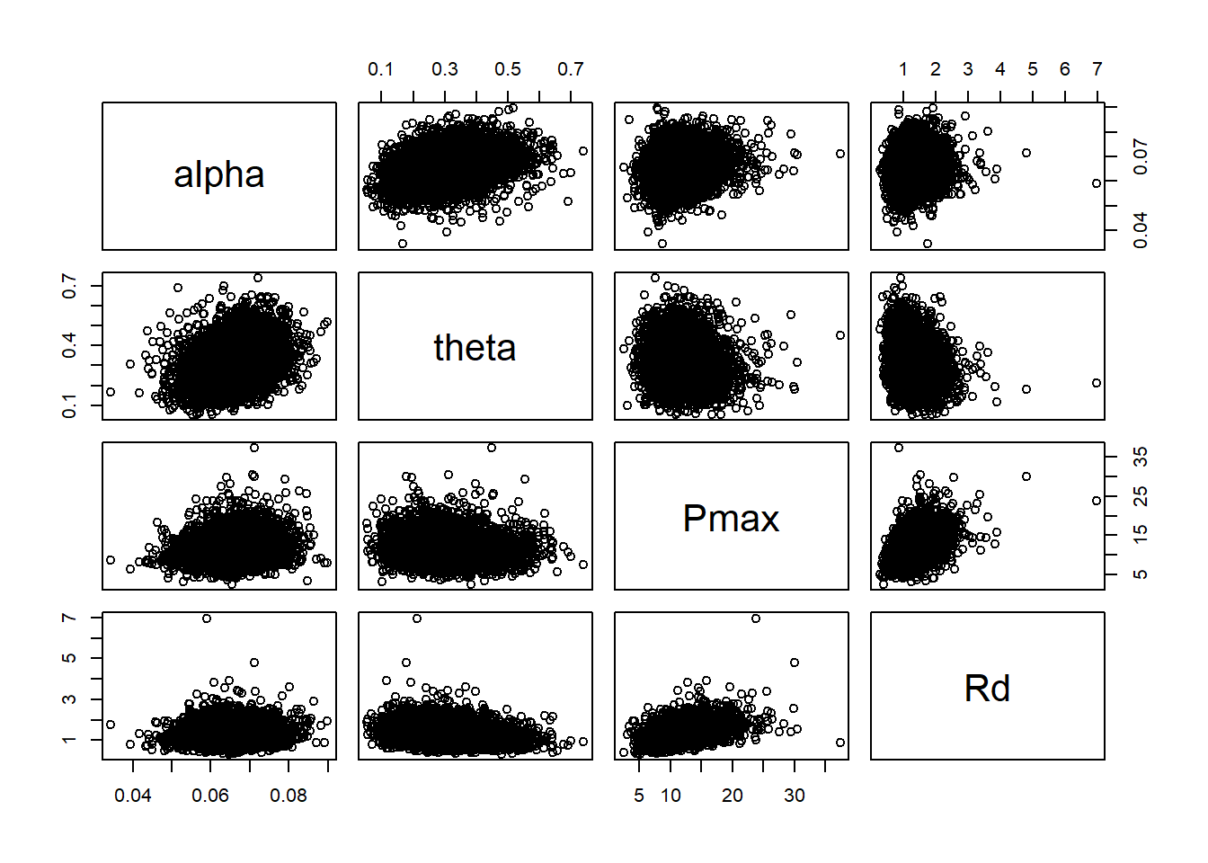
If you want to compare the models with and without correlations you would use kfold() across Replicate in a similar way as we did for location in the irrigation example.