1 Statistical inference in R

Author

Alejandro Morales & Joost van Heerwaarden

1.1 R and RStudio

R is a powerful tool for data analysis and visualization. It is widely used in academia, industry, and government for a variety of applications, including statistical modeling, machine learning, and data visualization. R is open-source and freely available, which makes it accessible to anyone who wants to use it. R has a large and active community of users and developers, which means that there are many resources available to help you learn and use R effectively. R is also highly extensible, which means that you can easily add new functionality to R by installing packages that are available on the Comprehensive R Archive Network (CRAN) or other repositories.

One of the key features of R is its ability to create reproducible research. Reproducible research is the practice of making research methods and results transparent and accessible to others so that they can be verified and built upon but also useful to you in the future when you need to revisit your analysis. Programming languages like R are well-suited for reproducible research because they allow you to write code that is self-contained, modular, and customizable. This means that you can easily share your code and data with others, break your analysis into small, manageable pieces that are easier to understand and debug, and create high-quality graphics and analyses that are tailored to your needs.

1.1.1 RStudio

You do not have to use RStudio to use R, but it is highly recommended. RStudio is an integrated development environment (IDE) for R that provides a user-friendly interface for writing, running, and debugging R code. RStudio includes a code editor, a console for running R code, a workspace for viewing objects in memory, and a file browser for managing files and directories. RStudio also includes tools for creating and managing R projects, which helps to organize code, data, and output in a structured way.

1.1.2 R/RStudio projects

R projects are a way to organize your work. An R project is a directory that contains all of the files and data associated with a particular analysis or project. R projects are useful because they help to keep your work organized, make it easier to share your work with others, and make it easier to reproduce your work in the future. We recommend that you create an R project using RStudio although this is not strictly necessary.

Inside the directory of an R project, you can create subdirectories to keep files organized. We recommend the following folder structure for an R project:

data: This directory is used to store raw and processed data files that are used in the analysis. Never modify the raw data, so for that reason we recommend two subfolders named raw and processed. Keep the original data in the raw subfolder and save any clean data or intermediate results in the processed folder. R can read data in multiple formats, such as CSV, Excel, and text files, but we recommend using CSV files as much as possible. Make sure that the metadata of the data is stored in a separate file with an explanation of the variables and their units.
intermediate: This optional directory is used to store intermediate data files that are generated during the analysis. These files are used to store intermediate results of data cleaning, transformation, and processing steps or to store the results of intermediate analyses that are computationally expensive.
output: This directory is used to store figures and other outputs that are generated during the analysis. These are often the final products of the analysis and are used to communicate the results to others (e.g., in a report, paper or presentation).
scripts: This directory is used to store R scripts that contain the code for the analysis. A single script can be used to perform the entire analysis, or the analysis can be broken up into multiple scripts that are sourced from a main script. We recommend using a naming convention for scripts that includes a number to indicate the order in which they should be run (e.g., 01_data_cleaning.R, 02_modeling.R, 03_visualization.R although this will change depending on the context). Always include comments in the script to explain what each section of code does (for others and for your future self).

Exercise 1.1

Create an RStudio project for the first chapter of the course. Follow the guideliness listed above regarding the folder structure. The examples given for script files are probably not relevant for this chapter though, so feel free to come up with your own naming convention.

Solution 1.1

Open RStudio and create a new project by clicking on File -> New Project -> New Directory -> Empty Project.
Choose a name for the project (e.g., Chapter_1) and a location on your computer.
Create the following folders in the project directory: data/raw, data/processed, output and scripts and intermediate.
Create a new R script in the scripts folder and save it with a suitable name.

1.2 Vectors

We can create vectors in R using the c() function. For example, to create a vector of the first five positive integers, we can use the following code:

x <- c(1, 2, 3, 4, 5)
x

[1] 1 2 3 4 5

We can also create a vector of the first five positive integers using the : operator that will generate all the values within a range of numbers:

x <- 1:5
x

[1] 1 2 3 4 5

If we want a sequence of numbers with a different step size, we can use the seq() function.

x <- seq(from = 1, to = 10, by = 2)
x

[1] 1 3 5 7 9

The arguments from, to, and by specify the starting value, ending value, and step size of the sequence, respectively. If we want to create a sequence of numbers in decreasing order, we can use a negative step size:

x <- seq(from = 10, to = 1, by = -1)
x

 [1] 10  9  8  7  6  5  4  3  2  1

This is equivalent to using the : operator with the numbers in reverse order:

x <- 10:1
x

 [1] 10  9  8  7  6  5  4  3  2  1

We can access the elements of a vector using square brackets. For example, to access the first element of the vector x, we can use the following code:

x[1]

[1] 10

We can also access multiple elements of a vector using a vector of indices. For example, to access the first and third elements of the vector x, we can use the following code:

x[c(1, 3)]

[1] 10  8

We can perform arithmetic operations on vectors. For example, to add two vectors element-wise, we can use the following code:

x <- c(1, 2, 3, 4, 5)
y <- c(6, 7, 8, 9, 10)
z <- x + y
z

[1]  7  9 11 13 15

We can also perform element-wise multiplication, division, and subtraction using the *, /, and - operators, respectively.

Exercise 1.2

Create a vector x with the first 10 positive integers.
Extract the odd elements from x.
Create a vector with the integers from -5 to 5.
The same as before but now in reverse order (from 5 to -5)
Calculate the ratio of the last two vectors.

Solution 1.2

We can use the : operator to create the vector x as follows:

x = 1:10

This is equivalent to using the seq function:

x = seq(from = 1, to = 10, by = 1)

The odd elements of x can be extracted by first creating a vector with the indices of the odd elements and then using this vector to extract the elements from x. We can do this as follows:

idx = seq(from = 1, to = length(x), by = 2)
x[idx]

[1] 1 3 5 7 9

Notice that we make the code dependent on the length of x so that it works for any vector.

We can create a vector with the integers from -5 to 5 using the : operator as follows:

x = -5:5

In order to create the vector in reverse order, we can just include the numbers in the opposite order in the : operator:

x = 5:-5

We can calculate the ratio of the two vectors by dividing them element-wise:

x = -5:5
y = 5:-5
z = x / y
z

 [1]  -1  -1  -1  -1  -1 NaN  -1  -1  -1  -1  -1

The NaN value is the result of dividing zero by zero. It is a special value that stands for “Not a Number” and is used to represent undefined or unrepresentable values.

1.3 Matrices

We can create matrices in R using the matrix function. For example, to create a 2x2 matrix with the values 1, 2, 3, and 4, we can use the following code:

X <- matrix(c(1, 2, 3, 4), nrow = 2, ncol = 2)
X

     [,1] [,2]
[1,]    1    3
[2,]    2    4

We can access the elements of a matrix using square brackets. For example, to access the element in the first row and first column of the matrix X, we can use the following code:

X[1, 1]

[1] 1

We can also access entire rows or columns of a matrix using square brackets. For example, to access the first row of the matrix X, we can use the following code:

X[1, ]

[1] 1 3

And to access the first column we can use the following:

X[, 1]

[1] 1 2

Notice that the result is a vector. If we want to keep the result as a matrix, we can use the drop = FALSE argument:

X[1, , drop = FALSE]

     [,1] [,2]
[1,]    1    3

We can perform arithmetic operations on matrices. For example, to add two matrices element-wise, we can use the following code:

X1 <- matrix(c(1, 2, 3, 4), nrow = 2, ncol = 2)
X2 <- matrix(c(5, 6, 7, 8), nrow = 2, ncol = 2)
X3 <- X1 + X2
X3

     [,1] [,2]
[1,]    6   10
[2,]    8   12

We can also perform element-wise multiplication, division, and subtraction using the *, /, and - operators, respectively.

We can turn a vector into a matrix using the matrix function passing the vector as input and specifying the dimensions of the matrix. For example, given a vector of length 6, we can create a 2x3 matrix as follows:

x <- 1:6
X <- matrix(x, nrow = 2, ncol = 3)
X

     [,1] [,2] [,3]
[1,]    1    3    5
[2,]    2    4    6

By default the matrix is filled column-wise but we could also fill it row-wise with the byrow argument:

X <- matrix(x, nrow = 2, ncol = 3, byrow = TRUE)
X

     [,1] [,2] [,3]
[1,]    1    2    3
[2,]    4    5    6

The matrix product (a topic to be discussed in more dtail later in the course) can be computed using the %*% operator. For example, to compute the product of the two matrices X1 and X2 created before, we can use the following code:

X3 <- X1 %*% X2
X3

     [,1] [,2]
[1,]   23   31
[2,]   34   46

To transpose a matrix (i.e. switch rows and collumns) , we can use the t() function. For example, to transpose the matrix X, we can use the following code:

t(X)

     [,1] [,2]
[1,]    1    4
[2,]    2    5
[3,]    3    6

Finally, the inverse of a square matrix (will also be discussed later in the course) can be computed using the solve() function. For example, to compute the inverse of the matrix X, we can use the following code:

solve(X3)

     [,1]  [,2]
[1,] 11.5 -7.75
[2,] -8.5  5.75

Notice that the matrix must be square for the inverse to exist. For example, the following code will produce an error since X is not square:

solve(X)

Error in solve.default(X): 'a' (2 x 3) must be square

If the matrix is singular (i.e., not invertible because the determinant is zero, see Appendix on Linear Algebra), the solve() function will produce an error. For example, the following code will produce an error since X is singular:

X <- matrix(c(1, 2, 1, 2), nrow = 2, ncol = 2)
solve(X)

Error in solve.default(X): Lapack routine dgesv: system is exactly singular: U[2,2] = 0

Notice that this error states that X is exactly singular. In practice, matrices may be numerically (or computationally) singular, which means that the determinant is very close to zero. In this case, the error message is different. For example:

X <- matrix(c(0,1,1e-16,2), nrow = 2, ncol = 2)
solve(X)

Error in solve.default(X): system is computationally singular: reciprocal condition number = 1.66667e-17

Note that it mentions the condition number of the matrix, which is a measure of how close the matrix is to being singular (it is more sensitive than using the determinant, but this is beyond the scope of the course).

Errors about singularity may show up when fitting an statistical model to data, for example, when your model is overparameterized or when the data is not informative enough. This is because most (linear) statistical models are fitted through a procedure that requires inverting a matrix.

Exercise 1.3

Create a matrix X with the first 20 positive integers (i.e., 1, 2, … 20) as a 5x4 matrix.
Extract the first row of the matrix and leave it as a matrix.
Extract the third column of the matrix and leave it as a matrix.
Try to invert the matrix X.
Compute the matrix-matrix product the transpose of X and itself. Try to invert this matrix

Solution 1.3

We can create the matrix X as follows:

x = 1:20
X = matrix(x,5,4)

We can extract the first row of the matrix X (and keep it is a matrix, i.e., a row-vector) as follows:

X[1,,drop=FALSE]

     [,1] [,2] [,3] [,4]
[1,]    1    6   11   16

We can extract the third column of the matrix X (and keep it is a matrix, i.e., a column-vector) as follows:

X[,3,drop=FALSE]

     [,1]
[1,]   11
[2,]   12
[3,]   13
[4,]   14
[5,]   15

We cannot invert the matrix X since it is not square. The error message from solve confirms this:

solve(X)

Error in solve.default(X): 'a' (5 x 4) must be square

We can compute the matrix-matrix product of the transpose of X and X as follows:

XtX = t(X) %*% X

This matrix is now square and we can try to invert it as follows:

solve(XtX)

Error in solve.default(XtX): system is computationally singular: reciprocal condition number = 4.00875e-20

Unfortunately, this matrix is singular and cannot be inverted.

1.4 Data Frames

Data frames are a fundamental data structure in R for storing tabular data. They are similar to matrices, but they can store different types of data in each column. When we read tabular data from a file or other external source, it will be stored as a data frame. This is also the format that most statistical models in R expect the data to be in. We can create data frames using the data.frame function. For example, to create a data frame with two columns x and y, we can use the following code:

df <- data.frame(x = c(1, 2, 3, 4, 5), y = c("a", "b", "c", "d", "e"))
df

We can access the columns of a data frame using the $ operator. For example, to access the column x of the data frame df, we can use the following code:

df$x

[1] 1 2 3 4 5

We can also access the columns of a data frame using double square brackets. For example, to access the column y of the data frame df, we can use the following code:

df[["y"]]

[1] "a" "b" "c" "d" "e"

Note that $ and [[]] can only access one column at a time and cannot be used to extract rows or individual values. If we want that, we can use square brackets indexing exactly as with matrices, with the addition that columns can be identified by their names and not just their position. For example:

df[1, "y"]

[1] "a"

and entire rows and columns can be extracted as well::

df[1, ] # 1st row

  x y
1 1 a

df[, 1] # 1st column

[1] 1 2 3 4 5

Notice that the result of extracting a column or row is a vector (just like with a matrix). If we want to keep the result as a data frame, we can use the drop = FALSE argument:

df[1, , drop = FALSE]

  x y
1 1 a

There are special functions to access the first or last rows of a data frame. For example, to access the first 5 rows of the data frame df, we can use the following code:

head(df, 5)

we can also access the last 5 rows of the data frame df using the following code:

tail(df, 5)

Note that the head() and tail() functions are useful when working with large data frames as otherwise R will try to print all the data to the screen. Also, the default number of rows is 5 so you can omit the second argument unless you want to specify a different number of rows.

1.5 Reading data from a file or website

1.5.1 CSV files

If you data is stored as a CSV file (recommended) we can read it using the read.csv() function. The argument to the function should be the path of the file in quotes, either on a hard drive or on the internet. When reading from a hard drive, the path should be relative to the working directory of the R session. If you are using an R project as explained in Chapter 1, the working directory will be the root of the project where the .Rproj file is located.

For example to read a CSV we just pass the address where the file is located. For example, the following will retrieve a dataset of trees from John Burkardt’s website on file formats:

data <- read.csv("https://people.sc.fsu.edu/~jburkardt/data/csv/trees.csv")
head(data)

  Index Girth..in. Height..ft. Volume.ft.3.
1     1        8.3          70         10.3
2     2        8.6          65         10.3
3     3        8.8          63         10.2
4     4       10.5          72         16.4
5     5       10.7          81         18.8
6     6       10.8          83         19.7

In you open the file directly from the website you will see that it contains four columns with the first row reserved for the column names. This is called the header of the file and read.csv() will automatically use it to name the columns of the data frame.

If the file does not have a header, you can use the header = FALSE argument to read.csv() to specify that the first row should be treated as data and not as column names. If there is additional metadata in the file (for example, there are multiple lines at the beginning of the file that are not part of the data), you can use the skip argument to read.csv() to specify how many lines to skip at the start of the file.

If you compare the names of the columns in data with the original file, you will see that R has removed the spaces and brackets and replaced them with dots. This is because R does not allow spaces or special characters in column names (only digits, letters, dots and underscores). It will also remove the quotes (") from the name (if present). They will be added back when printing the names of the columns (to denote that they are characters and not numbers):

colnames(data) # Extract the column names in data

[1] "Index"        "Girth..in."   "Height..ft."  "Volume.ft.3."

Although it is possible to use header and skip and to rename the columns, it is usually easier to adapt the file to the needs of R before reading it, so please make sure that the raw data is formatted appropiately before starting your analysis. In this case we cannot do this since the data is hosted online, but we can rename the columns in R:

colnames(data) <- c("Index", "Girth", "Height", "Volume")
head(data)

  Index Girth Height Volume
1     1   8.3     70   10.3
2     2   8.6     65   10.3
3     3   8.8     63   10.2
4     4  10.5     72   16.4
5     5  10.7     81   18.8
6     6  10.8     83   19.7

1.5.2 Other file formats

R can read many other file formats, including Excel or other plain text formats such as tab-separated or space-separated files. For plain text files you can use read.table() with the sep argument to specify the separator character. For example, to read a tab-separated file, you can use the following code:

data <- read.table("path/to/file.txt", sep = "\t")

In fact, read.csv() is just a wrapper around read.table() with the sep argument set ",", so we can also specify the arguments header and skip in read.table().

For Excel you will need to use a dedicated package such as readxl or openxlsx. However, we recommend converting the Excel file to a CSV file before reading it in R and make sure that the file is properly formatted (no merged cells, no empty rows or columns, no special characters in the column names, etc.). When converting Excel to CSV be careful with the locale settings of your computer, make sure that decimal digits are separated with a dot (.) and not a comma. If not possible, make sure that Excel uses a ";" as separator and read the file using sep = ";" in read.table() or use read.csv2().

1.5.3 Data in R packages

Many R packages come with datasets that can be used to test the functions in the package or to illustrate concepts. For example, the datasets package that comes with R has a dataset called trees that contains the growth of orange trees. We can load this dataset using the data() function:

data(Orange)
head(Orange)

  Tree  age circumference
1    1  118            30
2    1  484            58
3    1  664            87
4    1 1004           115
5    1 1231           120
6    1 1372           142

1.5.4 Create a data frame from scratch

If you want to create a data frame from scratch, you can use the data.frame() function. For example, to create a data frame with three columns N, Year, and Yield, we can use the following code:

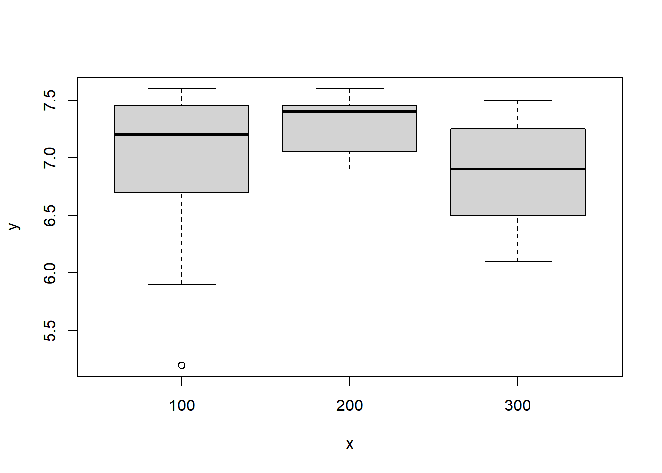
N = rep(c(50, 100, 150), each = 9)
yields <- data.frame(N = N,
                    Year = rep(2010:2012, each = 3),
                    Yield = rnorm(27, mean = 0.1*N, sd = 2))
head(yields, 5)

   N Year    Yield
1 50 2010 4.750504
2 50 2010 1.648153
3 50 2010 5.714475
4 50 2011 6.268409
5 50 2011 7.725407

In this example, we use the rep() function to create a vector N with the values 50, 100, and 150 repeated 9 times each. We then use the data.frame() function to create a data frame yields with the columns N, Year, and Yield. The Year column is created by repeating the values 2010, 2011, and 2012 three times each. Notice that the vector rep(2010:2012, each = 3) is actually too short to fill the column, but R will recycle the values as needed. The Yield column is created by generating 27 random numbers from a normal distribution with mean 0.1*N and standard deviation 2.

1.6 Working with data frames

We can summarize the contents of a data.frame by using the summary function. This will output a summary of the data in each column:

summary(data)

     Index          Girth           Height       Volume     
 Min.   : 1.0   Min.   : 8.30   Min.   :63   Min.   :10.20  
 1st Qu.: 8.5   1st Qu.:11.05   1st Qu.:72   1st Qu.:19.40  
 Median :16.0   Median :12.90   Median :76   Median :24.20  
 Mean   :16.0   Mean   :13.25   Mean   :76   Mean   :30.17  
 3rd Qu.:23.5   3rd Qu.:15.25   3rd Qu.:80   3rd Qu.:37.30  
 Max.   :31.0   Max.   :20.60   Max.   :87   Max.   :77.00

What is displayed depends on the type of data:

For numerical data, it will show the minimum, first quartile, median, mean, third quartile, and maximum.
For categorical data, it will show the number of times each category appears.
For factors, it will show the levels of the factor and the number of times each level appears.

We can check the data of each column by applying the class function to each column:

sapply(data, class)

    Index     Girth    Height    Volume 
"integer" "numeric" "integer" "numeric"

Here the sapply function is applying the class function to each column of the data frame data. You could replace class with any other function that you want to apply to each column in a data frame.

We can use the plot function to create a scatter plot of every two columns in the data frame:

plot(data)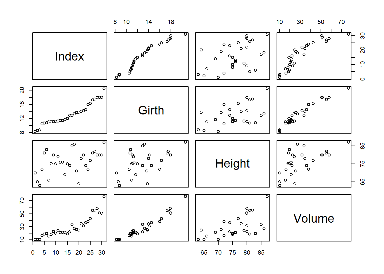

If we want to just plot two specific columns, we can just select the columns we want to plot through the usual indexing methods:

plot(data$Girth, data$Height)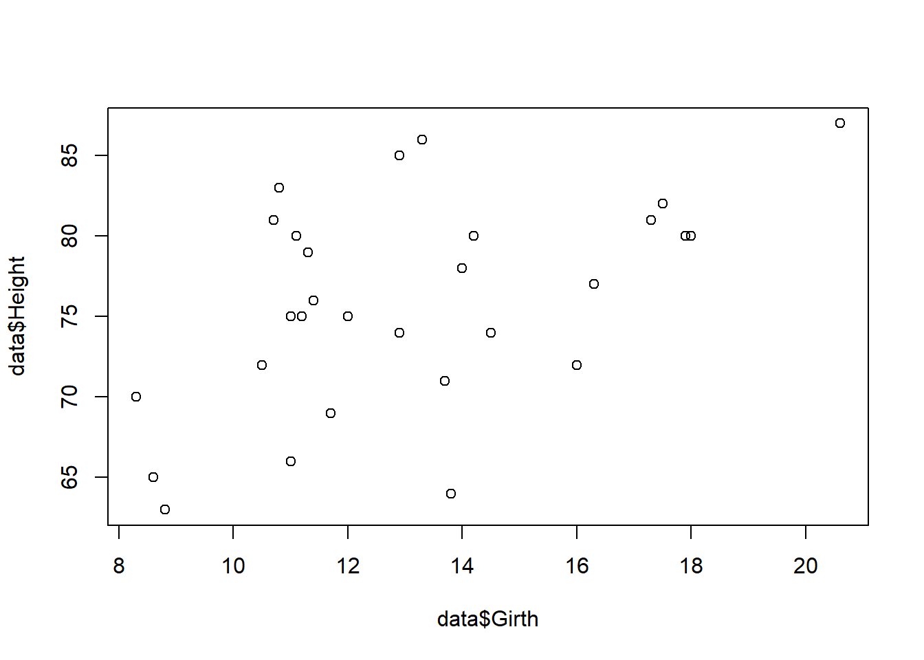

We can see that this kind easily get tedious because we have to type data$ every time we want to access a column. An alternative is to use the with function which allows us to write arbitary R code in a context where the columns of the data frame are directly accessible:

with(data, plot(Girth, Height))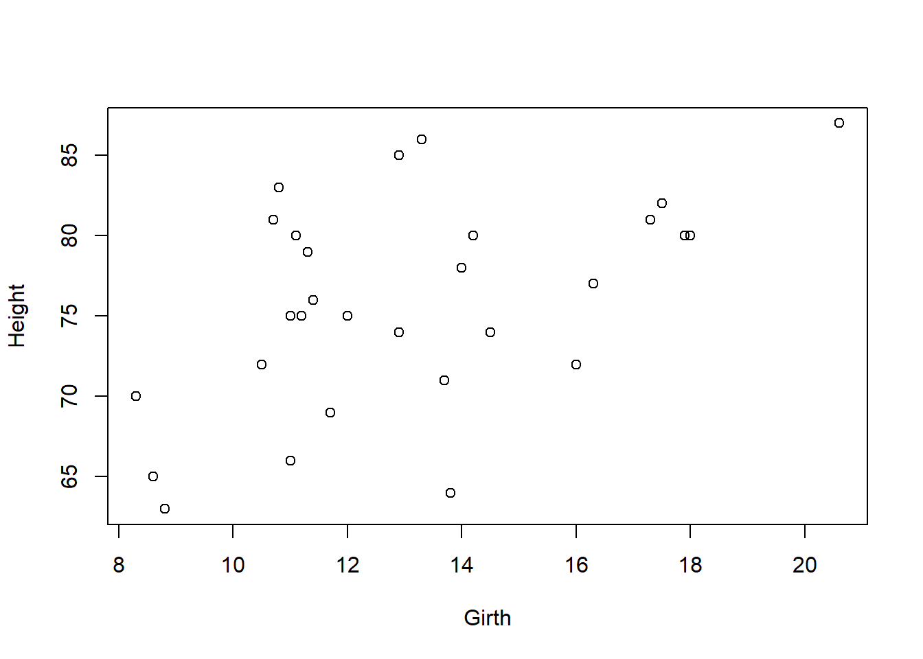

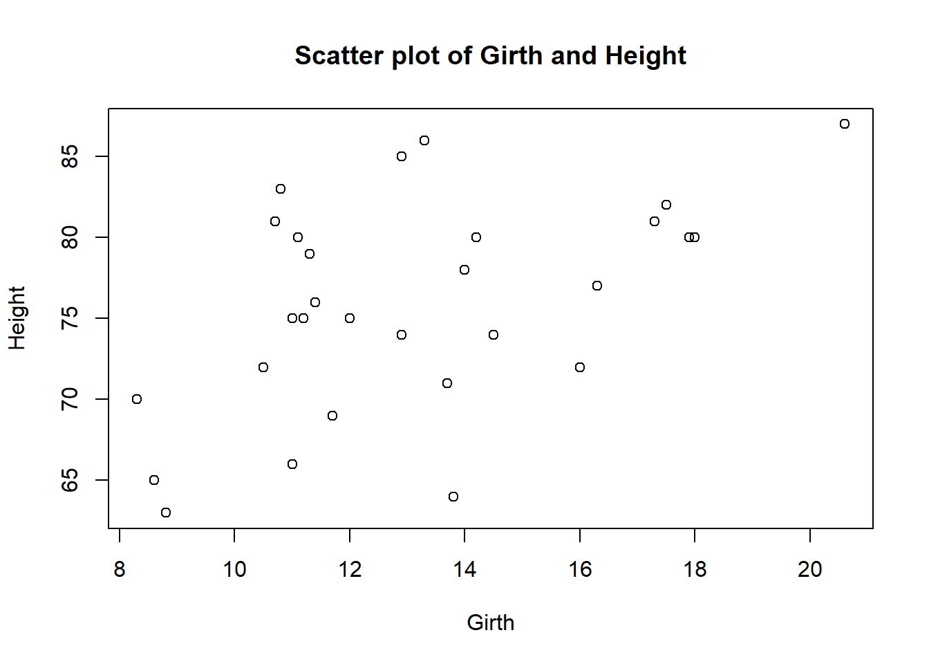
You can include multiple commands in the with function by separating them with commas or using curly brackets {}. For example, to create a scatter plot of Girth and Height and then add a title to the plot, we can use the following code:

with(data, {
    plot(Girth, Height)
    title("Scatter plot of Girth and Height")
})

With this function you cannot modify the data.frame though, so it is only useful for reading the data. If you want to modify the data, you can use the transform function to create a new data frame with the modified data. It is better to give the new data frame a different name to avoid confusion to avoid overwriting the original data. For example, to create a new column HGR with the ratio of Height and Girth we can use the following code:

new_data <- transform(data, HGR = Height/Girth)
head(new_data)

  Index Girth Height Volume      HGR
1     1   8.3     70   10.3 8.433735
2     2   8.6     65   10.3 7.558140
3     3   8.8     63   10.2 7.159091
4     4  10.5     72   16.4 6.857143
5     5  10.7     81   18.8 7.570093
6     6  10.8     83   19.7 7.685185

with(new_data, hist(HGR)) # Generate a histogram of the new column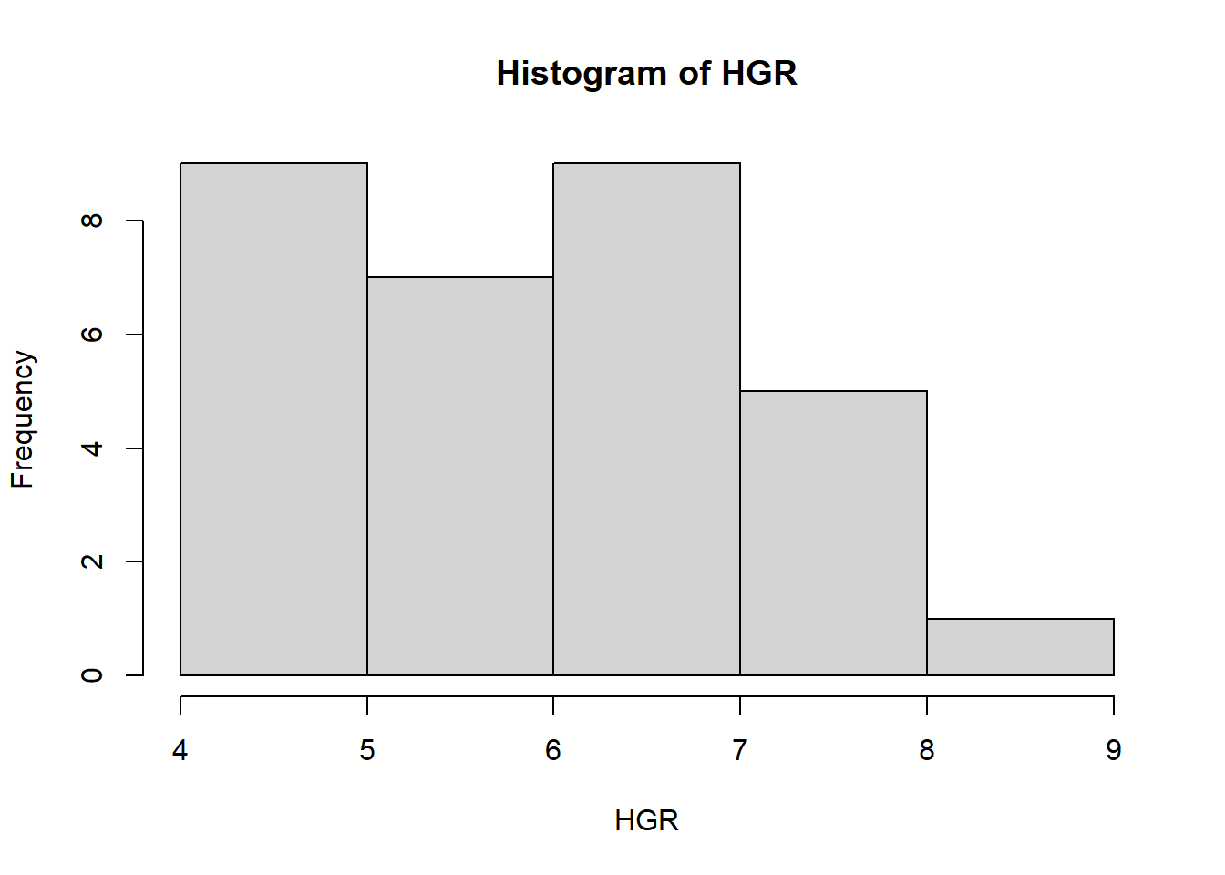

Most of the times we will not need to change the class of a column, but if we do, we can use the as function. For example, to change the class of the Girth column to a factor, we can use the as.factor function:

new_yields <- transform(yields, N = as.factor(N), Year = as.factor(Year))
summary(new_yields)

   N       Year       Yield       
 50 :9   2010:9   Min.   : 1.286  
 100:9   2011:9   1st Qu.: 5.991  
 150:9   2012:9   Median : 9.952  
                  Mean   :10.010  
                  3rd Qu.:14.457  
                  Max.   :18.920

We can identify rows that match specific conditions using the which function. For example, to identify the rows where the Girth is greater than 18, we can use the following code:

idx <- which(data$Girth > 18)
data[idx, ]

   Index Girth Height Volume
31    31  20.6     87     77

We can also use the subset function to extract a subset of the data frame that matches specific conditions. For example, to remove the rows where the Girth is greater than 18, we can use the following code:

clean_data <- subset(data, Girth <= 18)

Exercise 1.4

Load the data stored in the OrangeTreeTrunks.csv file.
There is an extreme value in the TrunkDiameter column. Identify the row where this value is located and remove it from the data frame.
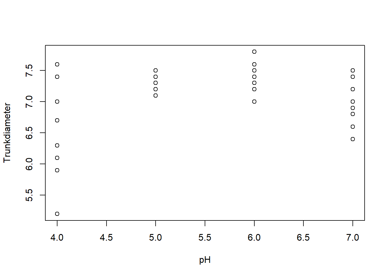
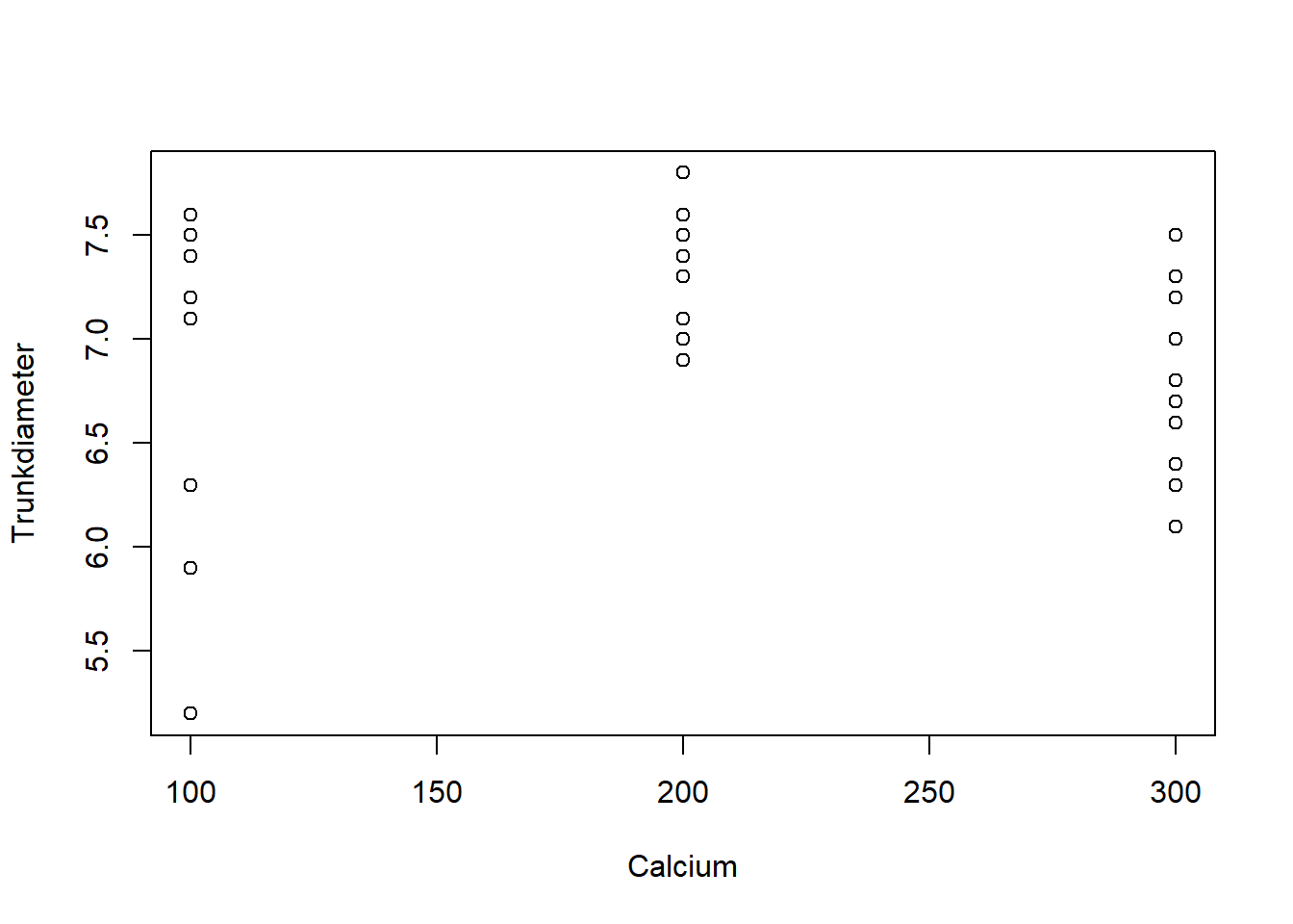
Plot the TrunkDiameter as a function of pH and Calcium treatments.
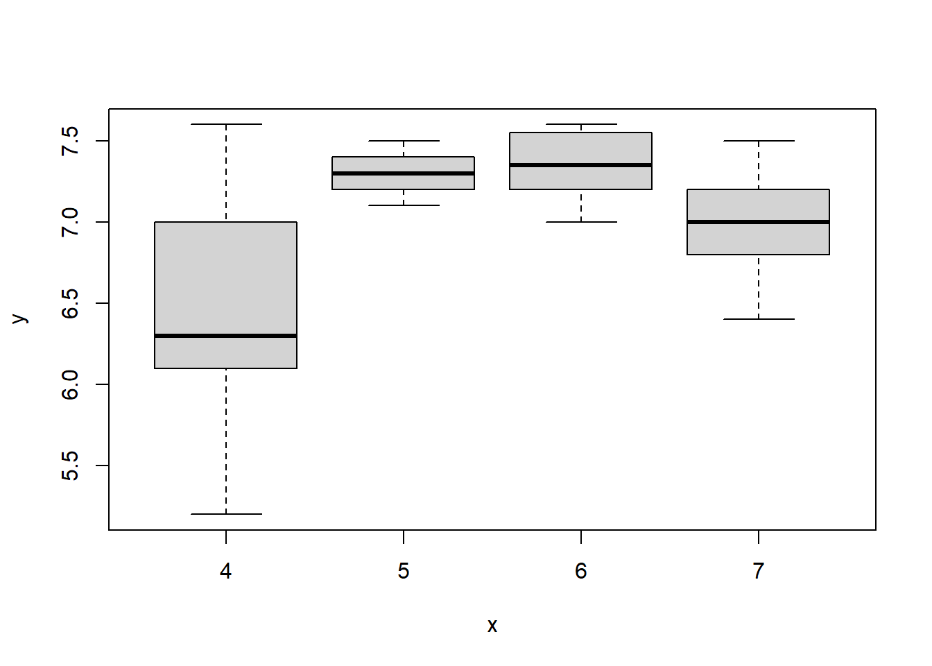
Convert the columns pH and Calcium to factors and redo the plots.
Make a histogram of the TrunkDiameter column.

Solution 1.4

We can read the data from the file by passing the correct path:

xp_data <- read.csv("data/raw/OrangeTreeTrunks.csv")

We can identify the row with the extreme value in the TrunkDiameter column using the which function:

idx <- which(xp_data$Trunkdiameter > 8)
xp_data[idx, ]

   pH Calcium Trunkdiameter
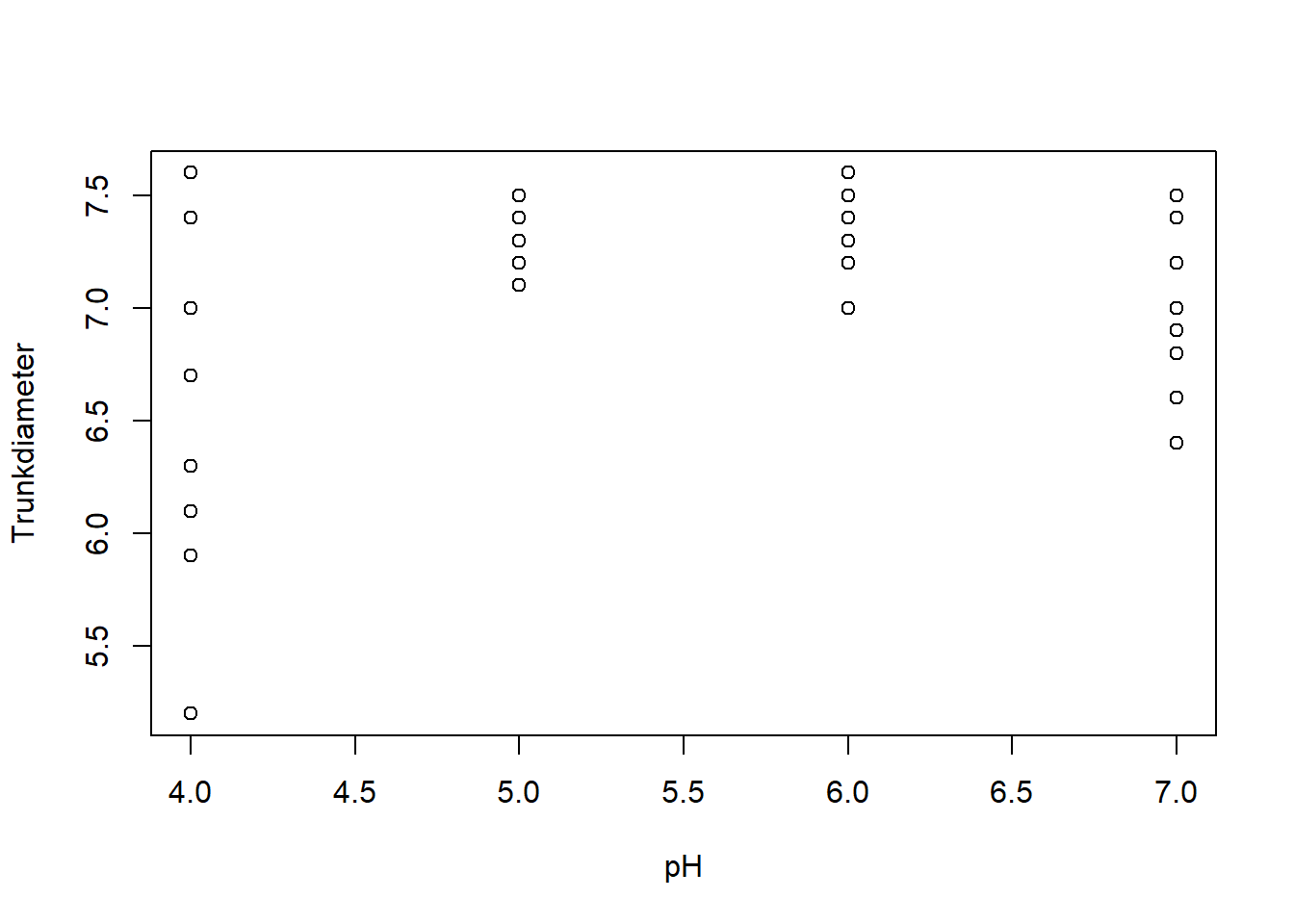
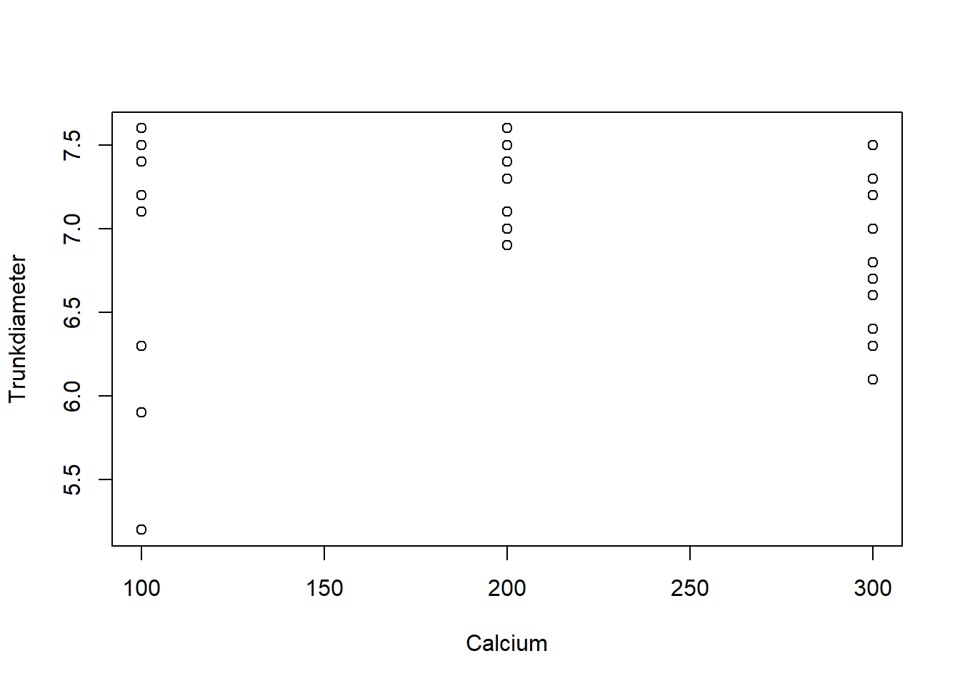
24  6     200            78

new_xp_data <- subset(xp_data, Trunkdiameter <= 8)

We can plot the TrunkDiameter as a function of pH and Calcium treatments using the with function:

with(new_xp_data,{
    plot(pH, Trunkdiameter)
    plot(Calcium, Trunkdiameter)
})

We can convert the columns pH and Calcium to factors using the as.factor function:

new_xp_data <- transform(new_xp_data,
                         pH = as.factor(pH),
                         Calcium = as.factor(Calcium))

We redo the plots:

with(new_xp_data,{
    plot(pH, Trunkdiameter)
    plot(Calcium, Trunkdiameter)
})

We can make a histogram of the TrunkDiameter column using the hist function:

hist(new_xp_data$Trunkdiameter)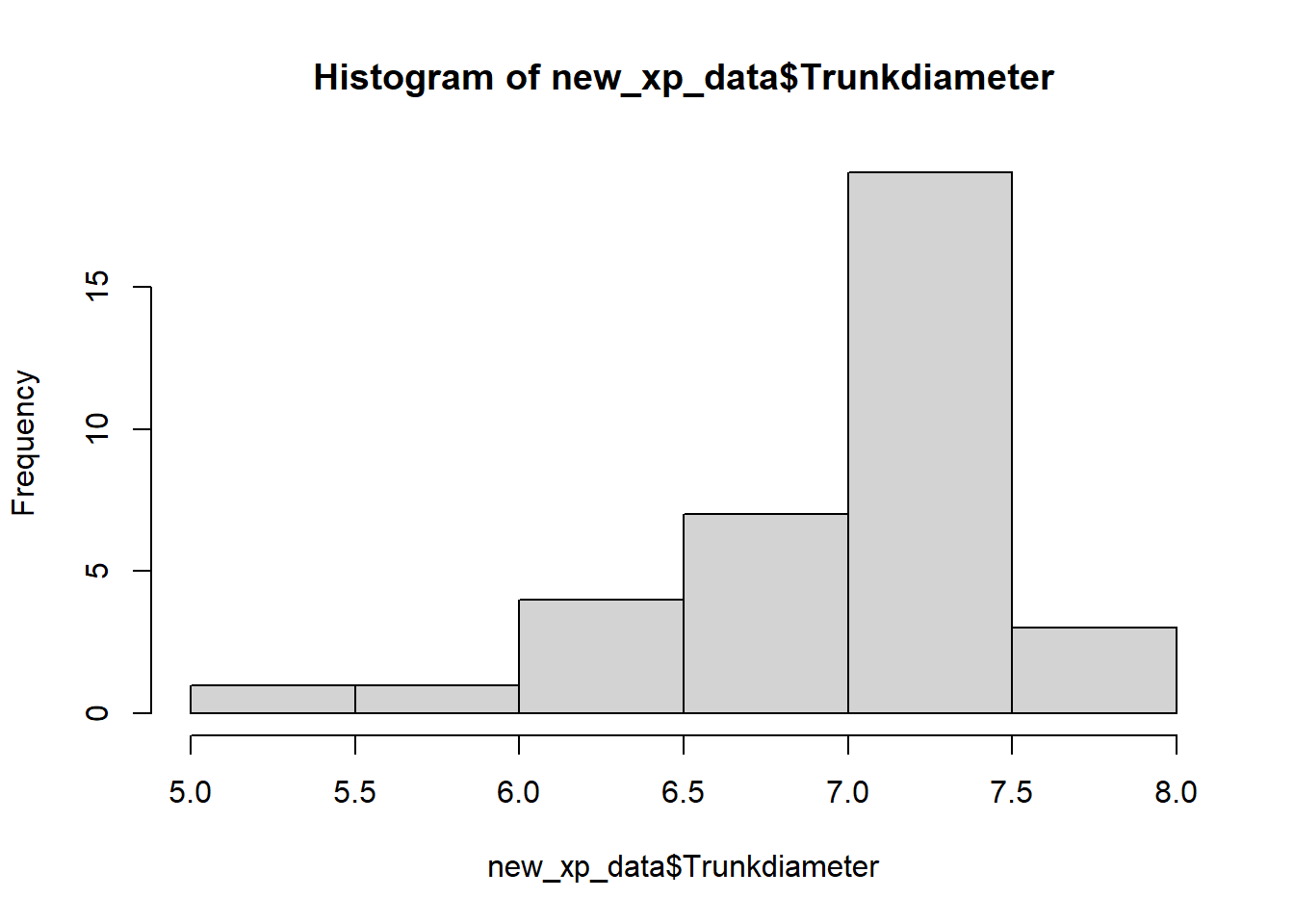

1.7 Saving results

We can save plots to a file using the pdf, png, or jpeg functions. For example, to save a plot to a PDF file, we can use the following code:

pdf("output/plot.pdf")
with(data, plot(Girth, Height))
dev.off()

To save a data frame (e.g. cleaned data) to a CSV file, we can use the write.csv function. For example,

write.csv(data, "output/data.csv", row.names = FALSE)

Finally, the sink function can be used to save the output of the R console to a file. For example, to save the output of the summary function to a text file, we can use the following code:

sink("output/summary.txt")
summary(data)
sink()

The sink is turned on the first time sink is called and turned off the second time. In the first call you can specify the file where the output will be saved. In the second call you do not need to specify a file, just call sink().

Exercise 1.5

Read the data stored in the OrangeTreeTrunks.csv file.
Identify the outlier in TrunkDiameter and fix its value (hint: there is a decimal digit missing).
Plot the TrunkDiameter as a function of pH and Calcium treatments.
Save the cleaned data to a CSV file in the appropiate folder.
Save the plots to PDF files in the appropiate folder.

Solution 1.5

We can read the data from the file by passing the correct path:

data <- read.csv("data/raw/OrangeTreeTrunks.csv")

We can identify the row with the extreme value in the TrunkDiameter column using the which function:

idx <- which(data$Trunkdiameter > 50)
data[idx, ]

   pH Calcium Trunkdiameter
24  6     200            78

clean_data <- data # Make a copy of the data to avoid modifying the original
clean_data$Trunkdiameter[idx] <- 7.8 # Should be 7.8 rather than 78

We can plot the TrunkDiameter as a function of pH and Calcium treatments using the plot function:

with(clean_data,{
    plot(pH, Trunkdiameter)
    plot(Calcium, Trunkdiameter)
})

We can save the cleaned data to a CSV file using the write.csv function:

write.csv(clean_data, "data/processed/clean_OrangeTreeTrunks.csv", row.names = FALSE)

We can save the plots to a PDF file using the pdf function:

pdf("output/TrunkDiameter_pH.pdf")
with(clean_data, plot(pH, Trunkdiameter))
dev.off()

png 
  2

pdf("output/TrunkDiameter_Calcium.pdf")
with(clean_data, plot(Calcium, Trunkdiameter))
dev.off()

png 
  2

1.8 Basics of statistical inference

1.8.1 Sampling from distributions in R

In R, we can represent a sample of values as a vector, where each element of the vector is an observation. To sample from a probability distribution we use the r functions, such as rnorm for the normal distribution (see Appendix on Distributions for more details). A sample of size $n = 10$ from a normal distribution with mean $\mu$ and standard deviation $\sigma$ can be generated as follows:

set.seed(0) # Make sure we always get the same results
n <- 10
mu <- 0
sigma <- 1
sample <- rnorm(n, mean = mu, sd = sigma)
sample

 [1]  1.262954285 -0.326233361  1.329799263  1.272429321  0.414641434
 [6] -1.539950042 -0.928567035 -0.294720447 -0.005767173  2.404653389

As discussed above, each value in the sample should be seen as an observation of a different random variable but in this case they are independent and identically distributed. This is equivalent to running rnorm $n$ times and storing the results in a vector through a for loop:

set.seed(0)
n <- 10
mu <- 0
sigma <- 1
sample <- numeric(n)
for(i in 1:n) {
    sample[i] <- rnorm(1, mean = mu, sd = sigma)
}
sample

 [1]  1.262954285 -0.326233361  1.329799263  1.272429321  0.414641434
 [6] -1.539950042 -0.928567035 -0.294720447 -0.005767173  2.404653389

The reason why we use the first approach is that it is more efficient and easier to read. However, it is important to keep in mind that each value in the sample is an observation of a different random variable and the values of mean and sd can change across observations. We can start relaxing the assumption of identical distribution by using different parameters for each observation. For example, we can generate a sample of size $n = 10$ from a normal distribution with a mean that increases linearly with the observation number:

set.seed(0)
n <- 10
mu <- 1:n # Vector from 1 to n
sigma <- 1
sample <- rnorm(n, mean = mu, sd = sigma)
sample

 [1]  2.262954  1.673767  4.329799  5.272429  5.414641  4.460050  6.071433
 [8]  7.705280  8.994233 12.404653

We can do the same with the standard deviation:

set.seed(0)
n <- 10
mu <- 1:n
sigma <- 1:n
sample <- rnorm(n, mean = mu, sd = sigma)
sample

 [1]  2.2629543  1.3475333  6.9893978  9.0897173  7.0732072 -3.2397003
 [7]  0.5000308  5.6422364  8.9480954 34.0465339

The one asusmption we cannot drop is the independence of the random variables from which the observations are taken. If we want to generate a sample of correlated random variables, we need to assume a multivariate distribution and generate the sample accordingly. We will show how to do this later.

Exercise 1.6

You are going to perform an experiment where you will measure the yield of a crop ($Y$ in t/ha) as a function of the amount of N it receives ($Y = 0.5 + 1.2N$). Assume that observations are subject to a measurement error and field-to-field variation, that follows a normal distribution with a standard deviation of 0.1 t/ha. Generate the data for the following scenarios (collect the data into a data frame so that we can analyze it later):

Assuming that the amount of N is fixed at 100 kg/ha, generate a sample of 10 observations of the yield of the crop.
Assuming that within an experiment the amount of N varies from 50 to 200 kg/ha in intevals of 50 kg/ha, simulate 10 replications per level of N.

Solution 1.6

To generate the data for the first scenario, we can use the following code:

sample = rnorm(10, mean = 0.5 + 1.2 * 100, sd = 0.1)
data_1 = data.frame(N = rep(100, 10), Y = sample)

Notice that we are using the formula $Y = 0.5 + 1.2N$ to calculate the mean of the normal distribution and the standard deviation is set to 0.1 t/ha to capture the measurement error.

In this case we are simulating 10 replicates, each of which has four observations (one for each value of N). The code to generate the data is as follows:

N = rep(c(50, 100, 150, 200), 10)
Y = rnorm(40, mean = 0.5 + 1.2 * N, sd = 0.1)
data_2 = data.frame(N = N, Y = Y, replicate = rep(1:10, each = 4))

This code generates the data for the second scenario. We first create a vector of N values that repeats each value four times (once for each observation). We then generate the yield values by sampling from a normal distribution with the mean calculated using the formula $Y = 0.5 + 1.2N$ and the standard deviation set to 0.1 t/ha. To keep track of the replicates, we add a column that repeats the numbers from 1 to 10 four times each.

1.8.2 Variance, covariance and correlation

See Appendix on statistical inference for details about these concepts.

Exercise 1.7

Generate three samples of size $n = 1000$ each, from three distributions:

A normal distribution with mean 100 and standard deviation 25 (call it sample_1).
A normal distribution with mean 100 and standard deviation 50 (call it sample_2).
The sample from point 1 plus a new sample from the same distribution (call it sample_3).
The sum of sample_1 and sample_3 (call it sample_4).

Visualize each sample with histogram.
Calculate the mean and variance of the first three samples and compare to theoretical value.
Calculate the covariance and correlation between each pair of samples. Use this to explain the variance of sample_4.
Generate a fourth sample as the sum of two samples from the first distribution (do not reuse previous samples). Calculate the correlation with respect to sample 1 and compare to results in the previous point.
Plot these samples against each other and interpret based on the correlations computed above.
Calculate the variance of 3 * sample_1 and compare to the theoretical value.

Solution 1.7

We can generate the first sample by calling rnorm() with the appropriate parameters but also setting the seed to ensure reproducibility:

set.seed(0)
n = 1e3
sample_1 <- rnorm(n, mean = 100, sd = 25)
sample_2 <- rnorm(n, mean = 100, sd = 50)
sample_3 <- sample_1 + rnorm(n, mean = 100, sd = 25)
sample_4 <- sample_1 + sample_3

We can visualize each sample with a histogram using the hist() function:

hist(sample_1)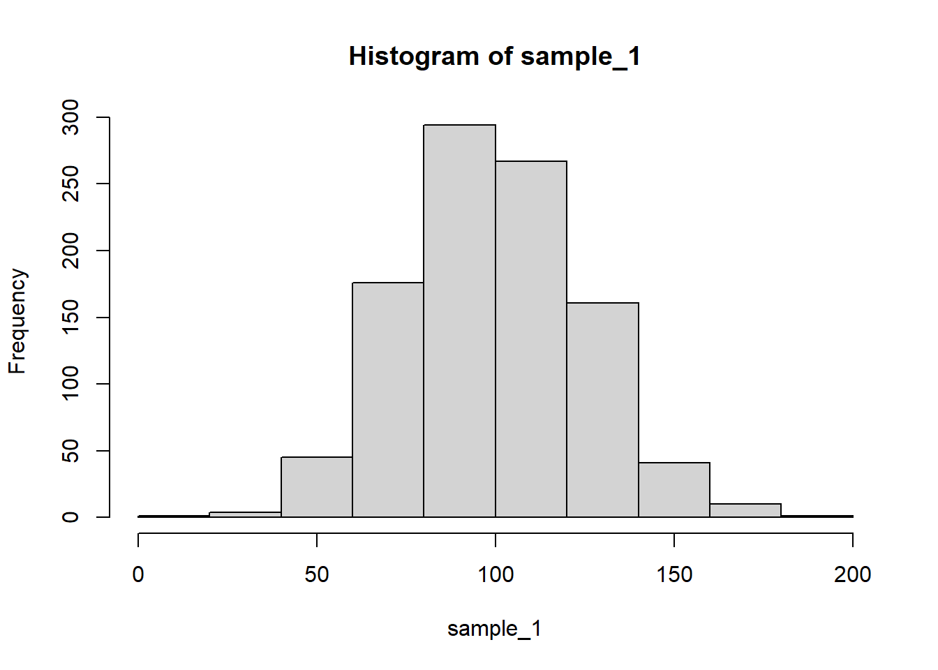

hist(sample_2)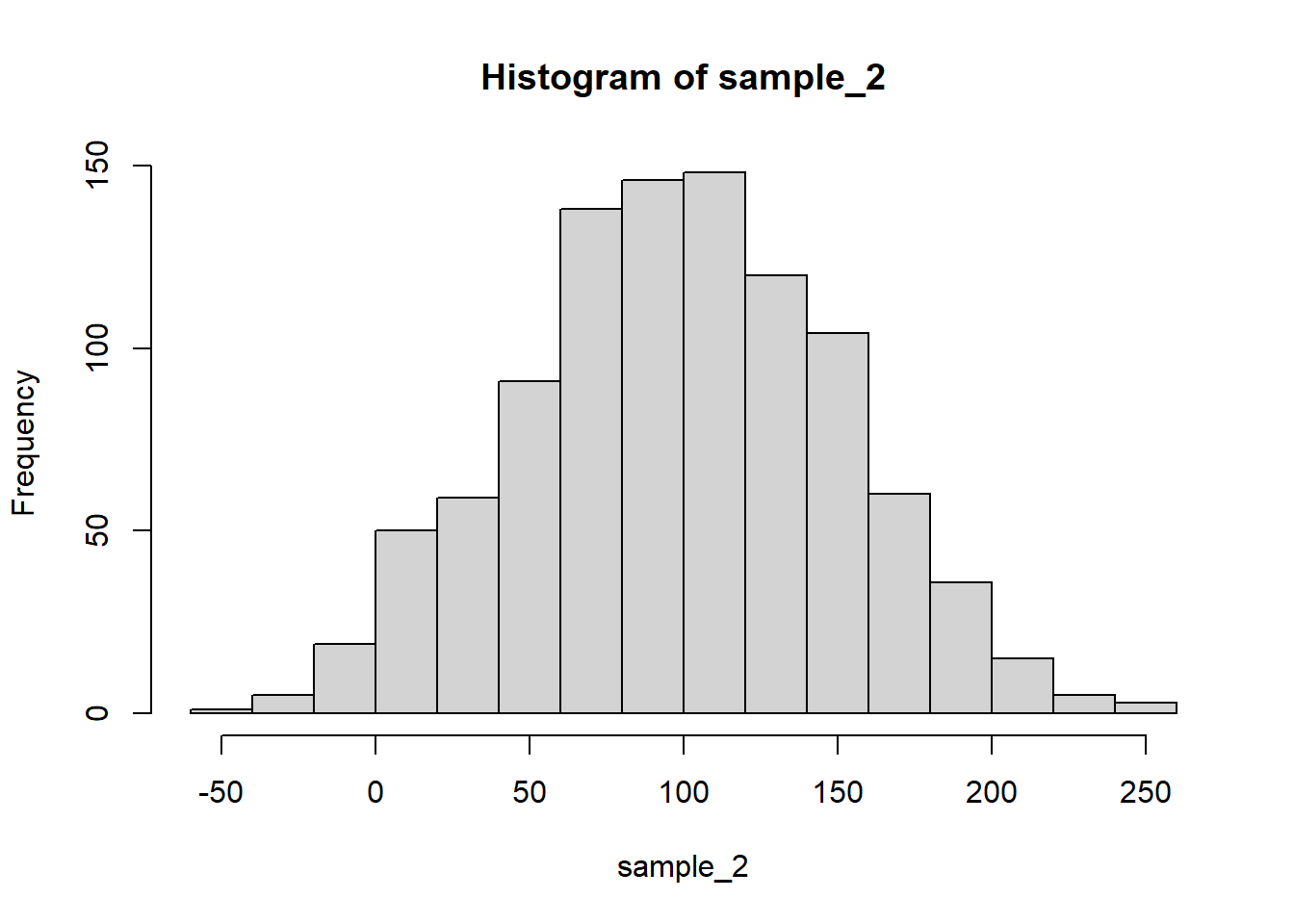

hist(sample_3)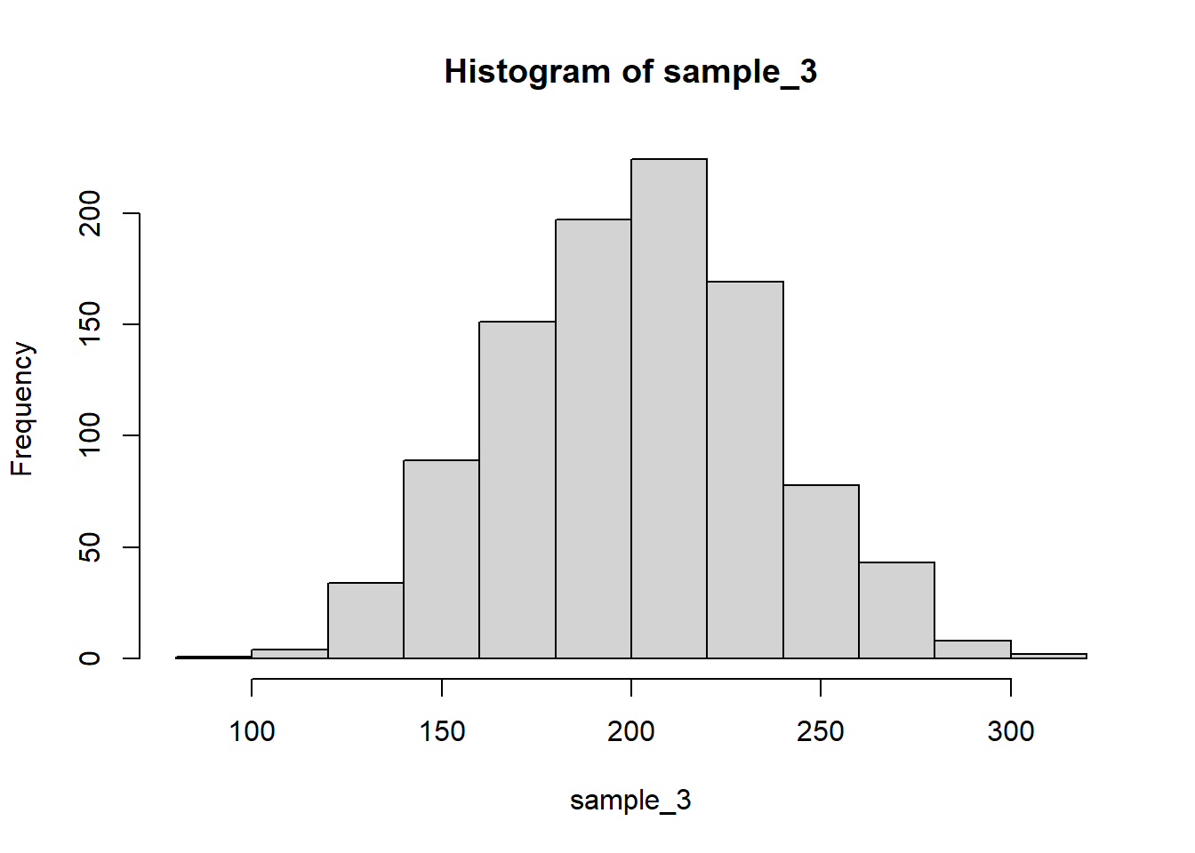

hist(sample_4)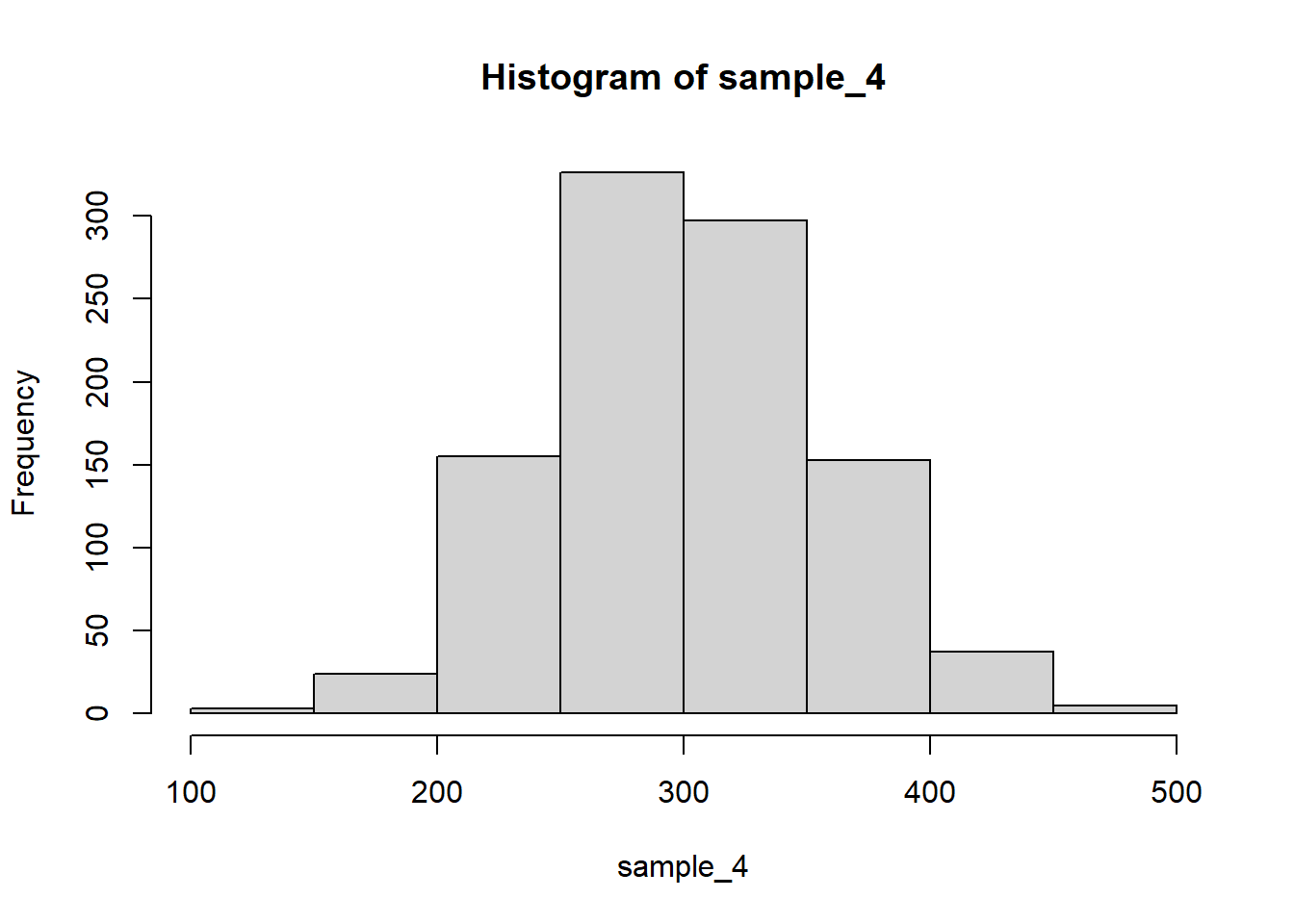

We can calculate the mean, variance and standard deviation of each sample using the mean() and var() functions:

mean(sample_1) # theory: 100

[1] 99.60426

var(sample_1) # theory: 25^2 = 625

[1] 622.5085

sd(sample_1) # theory: 25

[1] 24.95012

mean(sample_2) # theory: 100

[1] 98.76068

var(sample_2) # theory: 50^2 = 2500

[1] 2671.622

sd(sample_2) # theory: 50

[1] 51.68773

mean(sample_3) # theory: 100 + 100 = 200

[1] 201.3078

var(sample_3) # theory: 25^2 + 25^2 = 1250

[1] 1206.055

sd(sample_3) # theory: sqrt(1250) = 35.35534

[1] 34.7283

We can calculate the covariance and correlation between each pair of samples using the cov() and cor() functions:

cov(sample_1, sample_2) # theory: 0

[1] -16.27766

cor(sample_1, sample_2) # theory: 0

[1] -0.01262211

cov(sample_1, sample_3) # theory: != 0

[1] 629.6625

cor(sample_1, sample_3) # theory: != 0

[1] 0.7266941

cov(sample_2, sample_3) # theory: 0

[1] 9.122496

cor(sample_2, sample_3) # theory: 0

[1] 0.005082094

Notice how the covariance and correlation between the first two samples are different from the first and third samples. This is because the third sample is generated by adding to the first sample, which introduces a linear relationship between the two.

Let’s calculate the variance of the foruth sample:

var(sample_4) # theory: 25^2 + 25^2 + 2cov = 625 + 1250 + 2*622 = 3119

[1] 3087.889

Notice how the covariance now needs to be taken into account as sample_1 and sample_3 are nort independent.

We can generate the fourth sample as the sum of two samples from the first distribution:

sample_4 <- rnorm(n, mean = 100, sd = 25) + rnorm(n, mean = 100, sd = 25)
cor(sample_1, sample_4)

[1] -0.03538152

We can plot the first three samples against each other using the plot() function:

plot(sample_1, sample_2)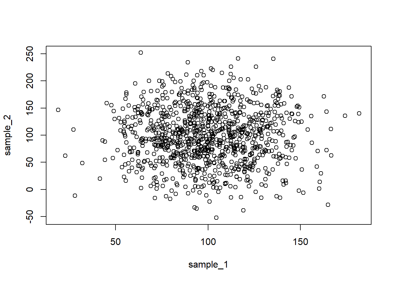

plot(sample_1, sample_3)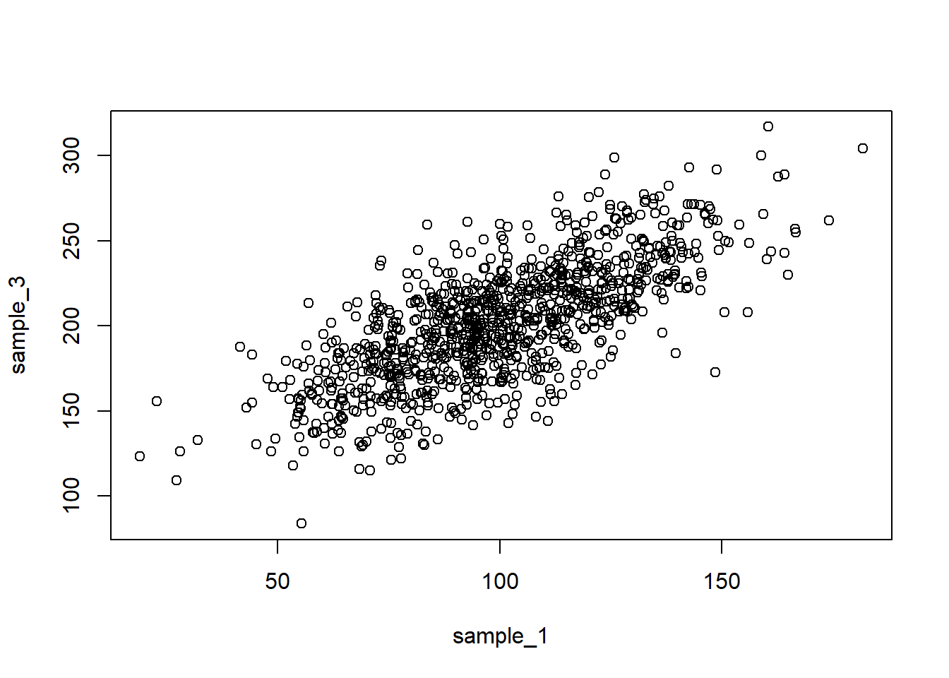

plot(sample_2, sample_3)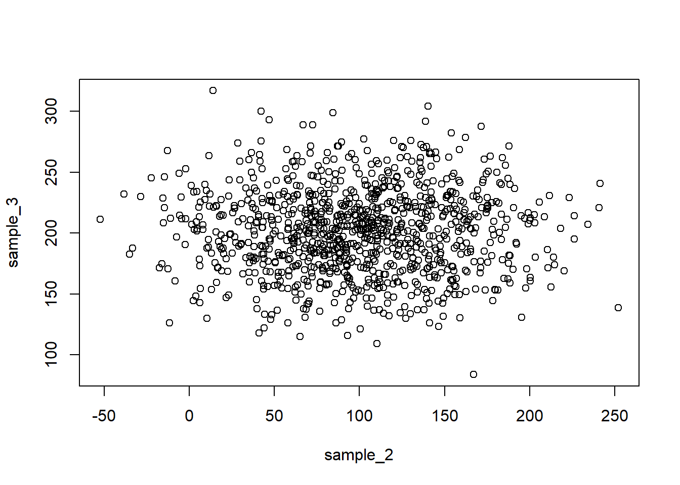

We can calculate the variance of 3 * sample_1 and compare to the theoretical value:

var(3 * sample_1) # theory: 3^2 * 25^2 = 3^2 * 625 = 5625

[1] 5602.577

Notice how the scaling factor is squared to determine the new variance.

1.8.3 Maximum likelihood estimation and ordinary least squares

We can use R to compute the log-likelihood function for a normal distribution. For example, if we have a sample of values $y$ and we want to estimate the mean of the population knowing that the standard deviation is 25, we can use the following code:

# Create the sample
set.seed(0)
n <- 100
y <- rnorm(n, mean = 100, sd = 25)
# Compute the log-likelihood for different values of mu
mu <- seq(70, 140, by = 1)
log_likelihood <- numeric(length(mu))
for(i in 1:length(mu)) {
    log_likelihood[i] <- sum(dnorm(y, mean = mu[i], sd = 25, log = TRUE))
}

We can visualize the log-likelihood function using the following code:

plot(mu, log_likelihood, type = "l", xlab = "Mean", ylab = "Log-likelihood")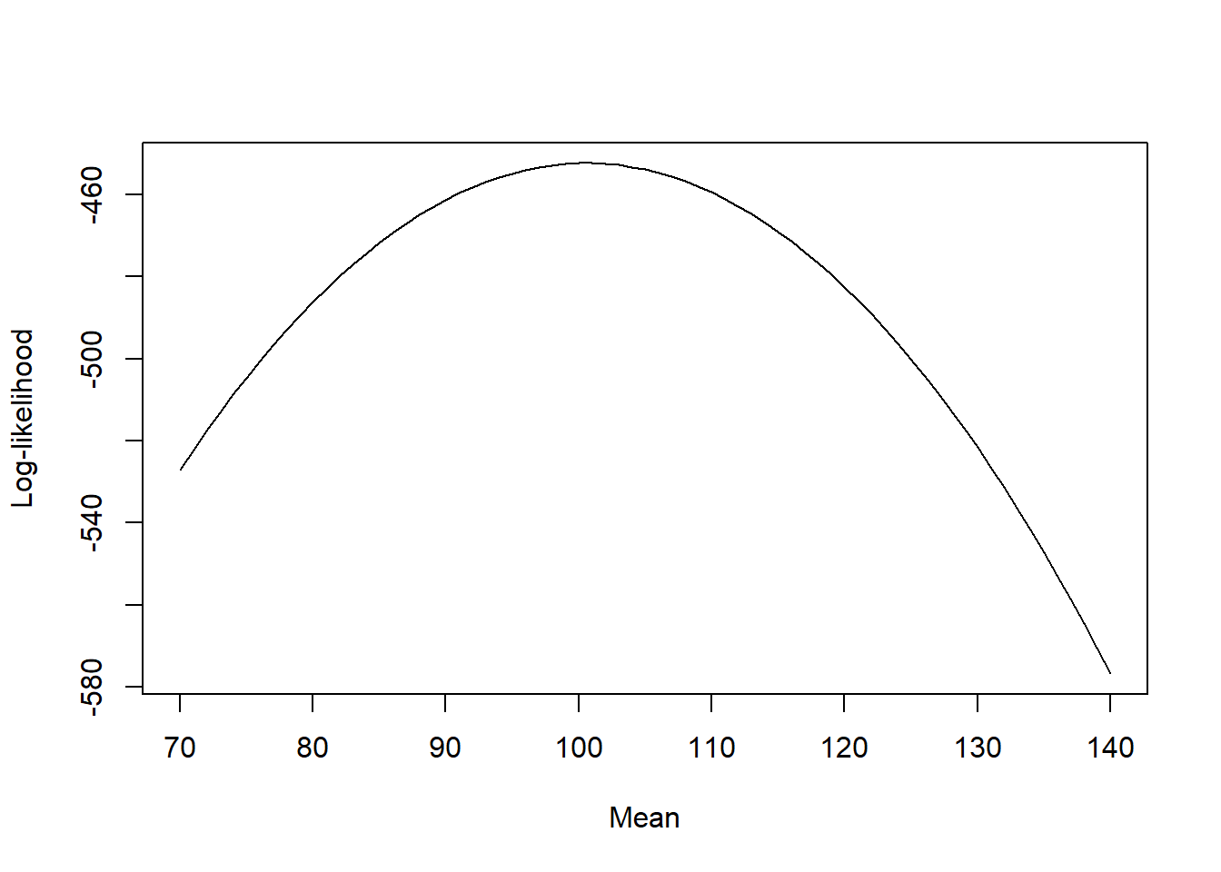

We can see that there is a maximum around 100, as expected. Do not worry about the actual values of the log-likelihood, only the shape of the curve is important and where the maximum is located.

We can compare this curve to the curve of the sum of squared errors:

# Compute the sum of squared errors for different values of mu
sse <- numeric(length(mu))
for(i in 1:length(mu)) {
    sse[i] <- sum((y - mu[i])^2)
}
plot(mu, sse, type = "l", xlab = "Mean", ylab = "Sum of squared errors")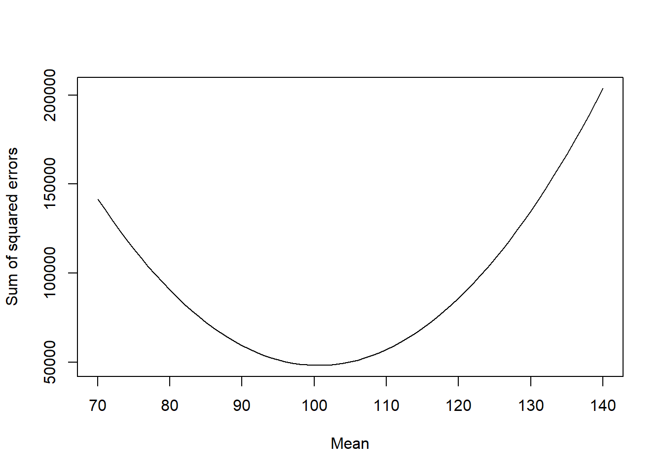

Notice that the shape of the curve is the same (though inverted, we maximize log-likelihood and minimize sum of squared errors), but the values are different (again the actual values are not relevant).

As we will see later, in most models we will compute the solution to this problem numerically through linear algebra, so we will not need to calculate these functions explicitly. There are cases where that is required (e.g., non-linear models) but for now this is just to show the connection between OLS and MLE and illustrate the conceptual procedure. That is, regardless of the implementation details, the goal is to find the parameters that maximize the likelihood of the data given the model.

Exercise 1.8

Explore the concept of maximum likelihood by simulating data from a binomial distribution and estimating the parameter pi (proportion). Use the following code, setting pi yourself:

####make a loop to estimate Pi by maximum likelihood (binomial distribution)
set.seed(0)
Pi=0.2 #choose your own value
n=10
y_obs<-rbinom(10,size=n,prob=Pi)

#proposed values of pi
prop_pi=seq(0.01,0.99,0.01)
#calculate Log Likelihoods for observed y (including observed)
LL.vec<-c() #vector for the likelihoods
#run a loop
for(i in 1:length(prop_pi)){
pp= prop_pi[i]  #proposed value 
LL<-sum(dbinom(y_obs,size=n,prob= pp,log = T)) #calculate the log likelihood
LL.vec[i]<-LL
}

visualize the results with a barplot (barplot(LL.vec~ prop_pi)
Identify the value of Pi that corresponds to the maximum Log Likelihood (visually and by printing the corresponding value of “prop_pi”)
How would you have estimated Pi from the vector of simulated values without using likelihood? Calculate this value and compare to the ML estimate

Solution 1.8

barplot(LL.vec~ prop_pi)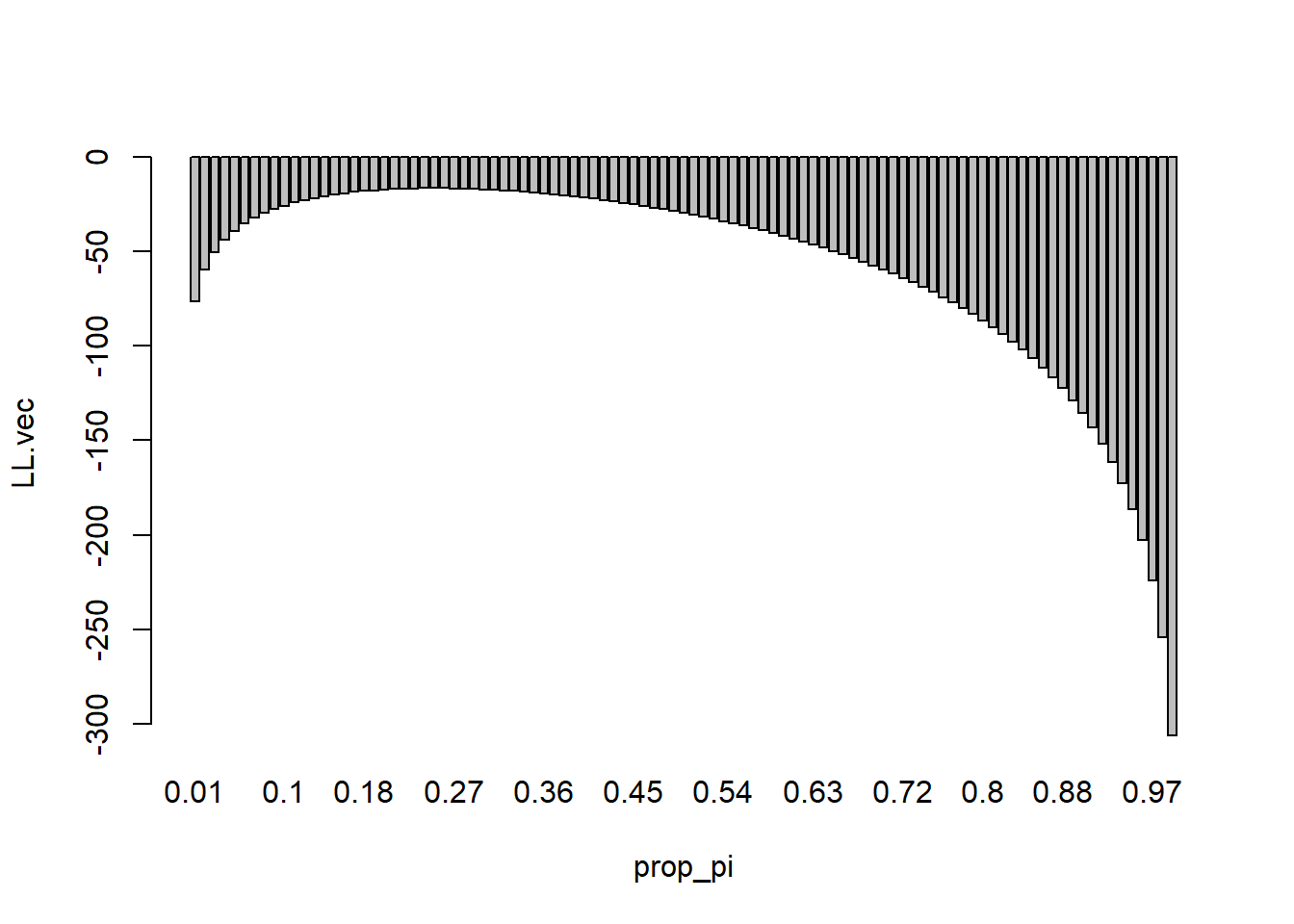

prop_pi[which(LL.vec==max(LL.vec))]

[1] 0.25

mean(y_obs)/n

[1] 0.25