n <- 5 # Number of replicates per level
data <- data.frame(G = as.factor(rep(1:3, each = n)),
                   y_true = NA,
y_obs = NA)3 General linear model II
3.1 General linear algebra
Please go to the appendix on Linear Algebra for a review of concepts in linear algebra and perform the exercises there.
3.2 Linear algebra behind linear models
3.2.1 Simulating data from a linear model
In order to illustrate the role that linear algebra plays in the context of linear models, we will consider a simple example with simulated data. Let’s assume that we have a dataset with a single categorical predictor variable with three levels, and a continuous response variable with 5 replicates per level. We first create the entries from the predictor and leave the repsonse variable empty:
Notice that we distinguish between the true response variable y_true and the observed response variable y_obs. The true response variable is generated from the predictor assuming coefficients \(\beta_0 = 1000\), \(\beta_1 = 10\), and \(\beta_2 = -5\) (one per level of the predictor variable):
beta <- c(1000, 10, -5)To compute y_true, we first create a design matrix X with the predictor variable G:
X <- model.matrix(~ G, data = data)Then, we compute the true response variable y_true as the product of the design matrix X and the coefficients beta:
data$y_true <- X %*% betaFinally, we add some random noise to the true response variable to obtain the observed response variable y_obs:
set.seed(123)
data$y_obs <- data$y_true + rnorm(nrow(data), mean = 0, sd = 100)
Let’s take a look at the data:
head(data) G y_true y_obs
1 1 1000 943.9524
2 1 1000 976.9823
3 1 1000 1155.8708
4 1 1000 1007.0508
5 1 1000 1012.9288
6 2 1010 1181.50653.2.2 Fitting a linear model
First let’s fit a linear model to the true response variable (so no observation errors):
fit_true <- lm(y_true ~ G, data = data)
summary(fit_true)
Warning in summary.lm(fit_true): essentially perfect fit: summary may be
unreliable
Call:
lm(formula = y_true ~ G, data = data)

Residuals:
       Min         1Q     Median         3Q        Max
-4.700e-13  0.000e+00  0.000e+00  5.733e-14  1.245e-13

Coefficients:
              Estimate Std. Error    t value Pr(>|t|)
(Intercept)  1.000e+03  6.785e-14  1.474e+16   <2e-16 ***
G2           1.000e+01  9.596e-14  1.042e+14   <2e-16 ***
G3          -5.000e+00  9.596e-14 -5.211e+13   <2e-16 ***
---
Signif. codes:  0 '***' 0.001 '**' 0.01 '*' 0.05 '.' 0.1 ' ' 1

Residual standard error: 1.517e-13 on 12 degrees of freedom
Multiple R-squared:      1, Adjusted R-squared:      1
F-statistic: 1.267e+28 on 2 and 12 DF,  p-value: < 2.2e-16
Of course the models fits perfectly (\(R^2\) of 1 and standard errors that are practically zero) and it recovers the exact coefficients. We can check the result of the summary by applying the internal linear algebra operation as shown in the lecture:
solve(t(X) %*% X) %*% t(X) %*% data$y_true [,1]
(Intercept) 1000
G2 10
G3 -5Let’s now fit a linear model to the observed response variable (with the error included):
fit_obs <- lm(y_obs ~ G, data = data)
summary(fit_obs)
Call:
lm(formula = y_obs ~ G, data = data)

Residuals:
    Min      1Q  Median      3Q     Max
-122.07  -53.31  -12.31   29.91  175.94

Coefficients:
            Estimate Std. Error t value Pr(>|t|)
(Intercept) 1019.357     40.169  25.376 8.52e-12 ***
G2           -13.789     56.808  -0.243    0.812
G3             6.433     56.808   0.113    0.912
---
Signif. codes:  0 '***' 0.001 '**' 0.01 '*' 0.05 '.' 0.1 ' ' 1

Residual standard error: 89.82 on 12 degrees of freedom
Multiple R-squared:  0.01091,   Adjusted R-squared:  -0.1539
F-statistic: 0.06615 on 2 and 12 DF,  p-value: 0.9363
Of course, now the model does not fit so well and the coefficients are not recovered exactly, although it still captures the orders of magnitude correctly. We can once again check the result of the summary by applying the internal linear algebra operation:
solve(t(X) %*% X) %*% t(X) %*% data$y_obs [,1]
(Intercept) 1019.357026
G2 -13.788923
G3 6.433147And we get exactly the same result as the summary. Notice that the linear algebra operation is the same for both cases, that is, the presence of errors in the response variable does not change the linear algebra operations that are performed to fit the model.
Let’s now compare the fitted values by the second model with the observations. In the previous chapter we learnt how to do this for each data point, but we can obtain all the fitted values in a single operation by using linear algebra:
y_fit <- X %*% coef(fit_obs)Notice that this is the same operation that was used to compute y_true in the first place, but now we are using the estimate of the coefficients rather than the true values. Of course, in practice you will just use predict() or fitted() to obtain the fitted values.
3.2.3 Computing the standard errors
To compute the standard errors of the parameter estimates we first need to calculate the residual standard error. The residuals are computed from the difference between the observed values and the fitted values (you could also run residuals(fit_obs) to get the same):
residuals <- data$y_obs - y_fitThe residual standard error can then be computed from these:
SSE <- sum(residuals^2)
df <- nrow(X) - ncol(X) # Degrees of freedom take from design matrix
RSE <- sqrt(SSE / df)
RSE
[1] 89.82163This is the same value that is reported in the summary of the model. Once we know RSE, we can now compute the covariance matrix of the model:
cov_matrix <- RSE^2 * solve(t(X) %*% X)
cov_matrix
(Intercept) G2 G3
(Intercept) 1613.585 -1613.585 -1613.585
G2 -1613.585 3227.170 1613.585
G3 -1613.585 1613.585 3227.170The standard errors of the coefficients are then the square root of the diagonal of this matrix:
se <- sqrt(diag(cov_matrix))
se
(Intercept) G2 G3
40.16945 56.80819 56.80819 Exercise 3.1
- Read the data from the file
Tilapia_growth.csvand make sure thatdietis encoded as a factor withControlas the first level. - Fit a linear model to the data including the interaction between
dietandsupplement. - Perform an ANOVA on the model to test the significance of the factors and their interaction.
- Verify the estimates of the coefficients and their standard errors by applying the linear algebra operations as shown in the lecture and above.
Solution 3.1
- We will now fit a linear model to a real dataset on growth of tilapia fish. The dataset represents the growth of tilapia fish as a function of different diets and supplements. Let’s first read the data:
dat<-read.csv("data/raw/Tilapia_growth.csv", header = T)
summary(dat)
Tank.nr. Treatment diet supplement
Min. : 1.00 Length:24 Length:24 Length:24
1st Qu.: 6.75 Class :character Class :character Class :character
Median :12.50 Mode :character Mode :character Mode :character
Mean :12.50
3rd Qu.:18.25
Max. :24.00
TW.initial..g. n.initial W.initial.g. n.final t
Min. :1205 Min. :30 Min. :40.20 Min. :28.00 Min. :42
1st Qu.:1223 1st Qu.:30 1st Qu.:40.80 1st Qu.:30.00 1st Qu.:42
Median :1234 Median :30 Median :41.10 Median :30.00 Median :42
Mean :1232 Mean :30 Mean :41.05 Mean :29.75 Mean :42
3rd Qu.:1240 3rd Qu.:30 3rd Qu.:41.30 3rd Qu.:30.00 3rd Qu.:42
Max. :1251 Max. :30 Max. :41.70 Max. :30.00 Max. :42
WG_total
Min. :48.20
1st Qu.:52.67
Median :55.55
Mean :56.63
3rd Qu.:61.45
Max. :66.20 Let’s make sure that diet is encoded as a factor and choose the levels to ensure the first one represents the control diet:
dat$diet <- factor(dat$diet, levels = c("Control","Citrus Pulp","Sunflower","Wheat Bran"))- The two factors in this experiment are
dietandsupplement. Let’s fit a complete model with the interaction between the two factors:
lm1 <- lm(WG_total ~ diet * supplement, data = dat)
summary(lm1)
Call:
lm(formula = WG_total ~ diet * supplement, data = dat)

Residuals:
    Min      1Q  Median      3Q     Max
-1.8333 -1.1083 -0.3333  1.0000  2.6667

Coefficients:
                                 Estimate Std. Error t value Pr(>|t|)
(Intercept)                       63.5333     0.9405  67.551  < 2e-16 ***
dietCitrus Pulp                   -9.4000     1.3301  -7.067 2.66e-06 ***
dietSunflower                    -13.7000     1.3301 -10.300 1.82e-08 ***
dietWheat Bran                    -7.3333     1.3301  -5.513 4.72e-05 ***
supplementEnzyme                  -0.3000     1.3301  -0.226   0.8244
dietCitrus Pulp:supplementEnzyme  -0.6667     1.8810  -0.354   0.7277
dietSunflower:supplementEnzyme     2.7333     1.8810   1.453   0.1655
dietWheat Bran:supplementEnzyme    4.8000     1.8810   2.552   0.0213 *
---
Signif. codes:  0 '***' 0.001 '**' 0.01 '*' 0.05 '.' 0.1 ' ' 1

Residual standard error: 1.629 on 16 degrees of freedom
Multiple R-squared:  0.9312,    Adjusted R-squared:  0.9011
F-statistic: 30.92 on 7 and 16 DF, p-value: 3.821e-08- The model is significant (F-statistic at the bottom of the summary) but it is hard to assess the significance of the diet or supplement effects due to the different levels of diet. Instead we should perform an ANOVA to test the significance of the factors:
anova(lm1)Analysis of Variance Table
Response: WG_total
Df Sum Sq Mean Sq F value Pr(>F)
diet 3 533.62 177.873 67.0272 2.811e-09 ***
supplement 1 12.04 12.042 4.5376 0.04903 *
diet:supplement 3 28.75 9.584 3.6115 0.03649 *
Residuals 16 42.46 2.654
---
Signif. codes: 0 '***' 0.001 '**' 0.01 '*' 0.05 '.' 0.1 ' ' 1- Let’s manually verify the estimates of the coefficients:
X <- model.matrix(~ diet * supplement, data = dat) # Design matrix from the formula
X
(Intercept) dietCitrus Pulp dietSunflower dietWheat Bran supplementEnzyme
1 1 1 0 0 1
2 1 1 0 0 0
3 1 0 1 0 0
4 1 0 0 1 0
5 1 0 0 1 1
6 1 0 0 0 1
7 1 0 1 0 1
8 1 0 0 0 0
9 1 0 1 0 0
10 1 0 0 0 1
11 1 1 0 0 0
12 1 1 0 0 1
13 1 0 0 1 1
14 1 0 0 0 0
15 1 0 1 0 1
16 1 0 0 1 0
17 1 0 0 0 0
18 1 1 0 0 1
19 1 1 0 0 0
20 1 0 0 1 0
21 1 0 0 0 1
22 1 0 0 1 1
23 1 0 1 0 0
24 1 0 1 0 1
dietCitrus Pulp:supplementEnzyme dietSunflower:supplementEnzyme
1 1 0
2 0 0
3 0 0
4 0 0
5 0 0
6 0 0
7 0 1
8 0 0
9 0 0
10 0 0
11 0 0
12 1 0
13 0 0
14 0 0
15 0 1
16 0 0
17 0 0
18 1 0
19 0 0
20 0 0
21 0 0
22 0 0
23 0 0
24 0 1
dietWheat Bran:supplementEnzyme
1 0
2 0
3 0
4 0
5 1
6 0
7 0
8 0
9 0
10 0
11 0
12 0
13 1
14 0
15 0
16 0
17 0
18 0
19 0
20 0
21 0
22 1
23 0
24 0
attr(,"assign")
[1] 0 1 1 1 2 3 3 3
attr(,"contrasts")
attr(,"contrasts")$diet
[1] "contr.treatment"
attr(,"contrasts")$supplement
[1] "contr.treatment"beta <- solve(t(X) %*% X) %*% t(X) %*% dat$WG_total
cbind(beta, coef(lm1)) [,1] [,2]
(Intercept) 63.5333333 63.5333333
dietCitrus Pulp -9.4000000 -9.4000000
dietSunflower -13.7000000 -13.7000000
dietWheat Bran -7.3333333 -7.3333333
supplementEnzyme -0.3000000 -0.3000000
dietCitrus Pulp:supplementEnzyme -0.6666667 -0.6666667
dietSunflower:supplementEnzyme 2.7333333 2.7333333
dietWheat Bran:supplementEnzyme 4.8000000 4.8000000The estimates are the same as in summary. We can also compute the standard errors:
residuals <- residuals(lm1)
SSE <- sum(residuals^2)
df <- nrow(X) - ncol(X) # Degrees of freedom take from design matrix
RSE <- sqrt(SSE / df)
cov_matrix <- RSE^2 * solve(t(X) %*% X)
se <- sqrt(diag(cov_matrix))
cbind(se, summary(lm1)$coefficients[,2])
se
(Intercept) 0.9405229 0.9405229
dietCitrus Pulp 1.3301002 1.3301002
dietSunflower 1.3301002 1.3301002
dietWheat Bran 1.3301002 1.3301002
supplementEnzyme 1.3301002 1.3301002
dietCitrus Pulp:supplementEnzyme 1.8810458 1.8810458
dietSunflower:supplementEnzyme 1.8810458 1.8810458
dietWheat Bran:supplementEnzyme 1.8810458 1.88104583.2.4 Estimating contrasts
In the previous chapter we learnt how to estimate contrasts between levels of a factor. We will show how the estimates and standard errors of these contrasts can be obtained from the linear algebra operations. Let’s first fit a model to the Tilapia data using Treatment as predictor:
dat <- read.csv("data/raw/Tilapia_growth.csv", header = T)
dat$Treatment <- as.factor(dat$Treatment)
lm1 <- lm(WG_total ~ Treatment, data = dat)
summary(lm1)
Call:
lm(formula = WG_total ~ Treatment, data = dat)

Residuals:
    Min      1Q  Median      3Q     Max
-1.8333 -1.1083 -0.3333  1.0000  2.6667

Coefficients:
                 Estimate Std. Error t value Pr(>|t|)
(Intercept)       63.5333     0.9405  67.551  < 2e-16 ***
TreatmentCON-ENZ  -0.3000     1.3301  -0.226    0.824
TreatmentCP-CON   -9.4000     1.3301  -7.067 2.66e-06 ***
TreatmentCP-ENZ  -10.3667     1.3301  -7.794 7.77e-07 ***
TreatmentSFM-CON -13.7000     1.3301 -10.300 1.82e-08 ***
TreatmentSFM-ENZ -11.2667     1.3301  -8.471 2.62e-07 ***
TreatmentWB-CON   -7.3333     1.3301  -5.513 4.72e-05 ***
TreatmentWB-ENZ   -2.8333     1.3301  -2.130    0.049 *
---
Signif. codes:  0 '***' 0.001 '**' 0.01 '*' 0.05 '.' 0.1 ' ' 1

Residual standard error: 1.629 on 16 degrees of freedom
Multiple R-squared:  0.9312,    Adjusted R-squared:  0.9011
F-statistic: 30.92 on 7 and 16 DF,  p-value: 3.821e-08
As an example, let’s compare the treatments with control diets vs the rest. First we check the levels of the factor:
levels(dat$Treatment)[1] "CON-CON" "CON-ENZ" "CP-CON" "CP-ENZ" "SFM-CON" "SFM-ENZ" "WB-CON"
[8] "WB-ENZ" All the treatment levels that start with CON are control diets. We can create a contrast matrix to compare these levels with the rest. This means comparing the mean of the first two levels with the mean of the other six levels. Remember that the indices in the contrast matrix refer to the coefficients in the model. The intercept of the model represents the mean of the first level whereas the rest of coefficients are the differences with respect to the first level. The contrast matrix is then:
C <- matrix(c(0,1/2,-1/6,-1/6,-1/6,-1/6,-1/6,-1/6), ncol = 1)
C
[,1]
[1,] 0.0000000
[2,] 0.5000000
[3,] -0.1666667
[4,] -0.1666667
[5,] -0.1666667
[6,] -0.1666667
[7,] -0.1666667
[8,] -0.1666667We can now compute the estimate of the contrasts with glht() from the multcomp package:
library(multcomp)Loading required package: mvtnormLoading required package: survivalLoading required package: TH.dataLoading required package: MASS
Attaching package: 'TH.data'The following object is masked from 'package:MASS':
geyserTestcontrast1<-glht(lm1,linfct= t(C))
summary(Testcontrast1)
     Simultaneous Tests for General Linear Hypotheses

Fit: lm(formula = WG_total ~ Treatment, data = dat)

Linear Hypotheses:
       Estimate Std. Error t value Pr(>|t|)
1 == 0   9.0000     0.7679   11.72  2.9e-09 ***
---
Signif. codes:  0 '***' 0.001 '**' 0.01 '*' 0.05 '.' 0.1 ' ' 1
(Adjusted p values reported -- single-step method)
Let’s now compute the estimate of the contrast manually from the linear algebra operations:
y=matrix(dat$WG_total,,1)
X<-model.matrix(lm1)
MSE<-sigma(lm1)^2
coef<-solve(t(X)%*%X)%*%t(X)%*%y
Estimate<-t(C)%*%coef
Estimate
[,1]
[1,] 9And the standard errors of the contrast:
COV<-MSE*t(C)%*%solve(t(X)%*%X)%*%C
SE<-sqrt(diag(COV))
SE
[1] 0.76793373.3 Generalized least squares
The generalized least squares allows for correlation among the residuals of different observations. This is implemented by a full covariance matrix instead of a single residual variance.
3.3.1 The linear model as a special case
The linear models fitted so far are a special case of the generalized least squares where the covariance matrix is diagonal with a constant variance (i.e., all covariances are zero). Let’s first revisit the linear model but using a full covariance matrix. First we fit model:
lm1 <- lm(WG_total~ Treatment,data=dat)
summary(lm1)
Call:
lm(formula = WG_total ~ Treatment, data = dat)

Residuals:
    Min      1Q  Median      3Q     Max
-1.8333 -1.1083 -0.3333  1.0000  2.6667

Coefficients:
                 Estimate Std. Error t value Pr(>|t|)
(Intercept)       63.5333     0.9405  67.551  < 2e-16 ***
TreatmentCON-ENZ  -0.3000     1.3301  -0.226    0.824
TreatmentCP-CON   -9.4000     1.3301  -7.067 2.66e-06 ***
TreatmentCP-ENZ  -10.3667     1.3301  -7.794 7.77e-07 ***
TreatmentSFM-CON -13.7000     1.3301 -10.300 1.82e-08 ***
TreatmentSFM-ENZ -11.2667     1.3301  -8.471 2.62e-07 ***
TreatmentWB-CON   -7.3333     1.3301  -5.513 4.72e-05 ***
TreatmentWB-ENZ   -2.8333     1.3301  -2.130    0.049 *
---
Signif. codes:  0 '***' 0.001 '**' 0.01 '*' 0.05 '.' 0.1 ' ' 1

Residual standard error: 1.629 on 16 degrees of freedom
Multiple R-squared:  0.9312,    Adjusted R-squared:  0.9011
F-statistic: 30.92 on 7 and 16 DF,  p-value: 3.821e-08
Let’s create the covariance matrix of the residuals. We need to create a matrix with the right dimensions and fill in the residual variance in the diagonal (this is equivalent to the mean squared error):
I <- diag(1,nrow(X))
S <- I * MSE
We can visualize the covariance matrix as a heatmap:
image(S)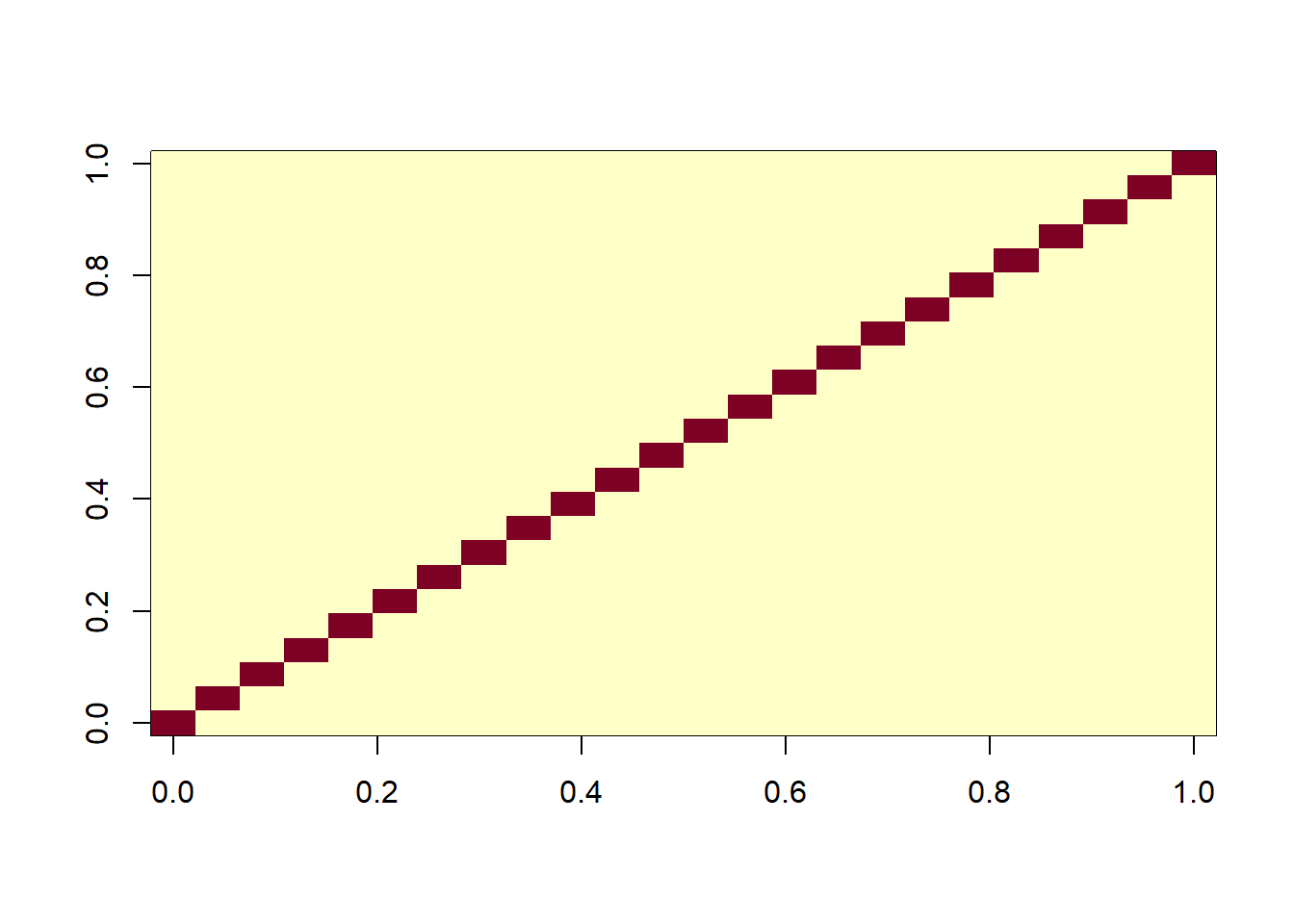
The coefficients are then estimated using the inverse of the covariance matrix:
S_inv<-solve(S)
coef<-solve(t(X)%*%S_inv%*%X)%*%t(X)%*%S_inv%*%y
coef
[,1]
(Intercept) 63.533333
TreatmentCON-ENZ -0.300000
TreatmentCP-CON -9.400000
TreatmentCP-ENZ -10.366667
TreatmentSFM-CON -13.700000
TreatmentSFM-ENZ -11.266667
TreatmentWB-CON -7.333333
TreatmentWB-ENZ -2.833333The standard errors are then computed also with the inverse of the covariance matrix:
COV_SE <- solve(t(X)%*%S_inv%*%X)
SE <- sqrt(diag(COV_SE))
matrix(SE, ncol = 1)
[,1]
[1,] 0.9405229
[2,] 1.3301002
[3,] 1.3301002
[4,] 1.3301002
[5,] 1.3301002
[6,] 1.3301002
[7,] 1.3301002
[8,] 1.33010023.3.2 Allowing for correlations among residuals
We are now going to modify the covariance matrix to allow for correlations among residuals within a treatment. We will assume that the residuals are correlated within a treatment but not between treatments:
# Set covariance within treatments to MSE/1.25
V2 <- matrix(MSE/1.25, nrow(X), nrow(X)) # Fill matrix with values
# Set covariance across treatments to zero
STM <- outer(dat$Treatment, dat$Treatment, "!=")
V2[STM] <- 0
# Set variances to MSE
diag(V2) <- MSE
V2[1:10, 1:10]
[,1] [,2] [,3] [,4] [,5] [,6] [,7] [,8] [,9]
[1,] 2.65375 0.00000 0.00000 0.00000 0.00000 0.00000 0.00000 0.00000 0.00000
[2,] 0.00000 2.65375 0.00000 0.00000 0.00000 0.00000 0.00000 0.00000 0.00000
[3,] 0.00000 0.00000 2.65375 0.00000 0.00000 0.00000 0.00000 0.00000 2.12300
[4,] 0.00000 0.00000 0.00000 2.65375 0.00000 0.00000 0.00000 0.00000 0.00000
[5,] 0.00000 0.00000 0.00000 0.00000 2.65375 0.00000 0.00000 0.00000 0.00000
[6,] 0.00000 0.00000 0.00000 0.00000 0.00000 2.65375 0.00000 0.00000 0.00000
[7,] 0.00000 0.00000 0.00000 0.00000 0.00000 0.00000 2.65375 0.00000 0.00000
[8,] 0.00000 0.00000 0.00000 0.00000 0.00000 0.00000 0.00000 2.65375 0.00000
[9,] 0.00000 0.00000 2.12300 0.00000 0.00000 0.00000 0.00000 0.00000 2.65375
[10,] 0.00000 0.00000 0.00000 0.00000 0.00000 2.12300 0.00000 0.00000 0.00000
[,10]
[1,] 0.00000
[2,] 0.00000
[3,] 0.00000
[4,] 0.00000
[5,] 0.00000
[6,] 2.12300
[7,] 0.00000
[8,] 0.00000
[9,] 0.00000
[10,] 2.65375Exercise 3.2
- Calculate the correlation coefficient between the residuals of the first two observations based on matrix
V2. - Generate a large sample of correlated residuals based on the covariance matrix
V2and compute the correlation coefficient numerically from the sample. - Estimate the coefficients and their standard errors from the linear model with the correlation matrix
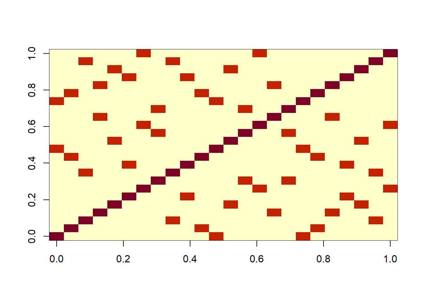
V2(GLS) and compare them with the estimates from the linear model with uncorrelated residuals (LM). - Visualize the covariance matrix
V2as a heatmap.
Solution 3.2
- The correlation coefficient is the covariance between the residuals of the first two observations divided by the product of the standard deviations of the residuals of the two observations. The covariance is the value in the matrix
V2at the index[1,2](or[2,1]). The standard deviations are the square root of the values in the diagonal of the matrixV2. The correlation coefficient is then:
V2[1,2]/(sqrt(V2[1,1])*sqrt(V2[2,2]))[1] 0- We can generate a large sample of residuals from the covariance matrix
V2and compute the correlation coefficient numerically. We first generate the residuals:
set.seed(123)
library(MASS) # Load library. If not installed, install it with install.packages("MASS")
MVmat <- rmvnorm(1e6, mean =rep(0,ncol(V2)), sigma = V2)
round(cor(MVmat),2)
[,1] [,2] [,3] [,4] [,5] [,6] [,7] [,8] [,9] [,10] [,11] [,12] [,13]
[1,] 1.0 0.0 0.0 0.0 0.0 0.0 0.0 0.0 0.0 0.0 0.0 0.8 0.0
[2,] 0.0 1.0 0.0 0.0 0.0 0.0 0.0 0.0 0.0 0.0 0.8 0.0 0.0
[3,] 0.0 0.0 1.0 0.0 0.0 0.0 0.0 0.0 0.8 0.0 0.0 0.0 0.0
[4,] 0.0 0.0 0.0 1.0 0.0 0.0 0.0 0.0 0.0 0.0 0.0 0.0 0.0
[5,] 0.0 0.0 0.0 0.0 1.0 0.0 0.0 0.0 0.0 0.0 0.0 0.0 0.8
[6,] 0.0 0.0 0.0 0.0 0.0 1.0 0.0 0.0 0.0 0.8 0.0 0.0 0.0
[7,] 0.0 0.0 0.0 0.0 0.0 0.0 1.0 0.0 0.0 0.0 0.0 0.0 0.0
[8,] 0.0 0.0 0.0 0.0 0.0 0.0 0.0 1.0 0.0 0.0 0.0 0.0 0.0
[9,] 0.0 0.0 0.8 0.0 0.0 0.0 0.0 0.0 1.0 0.0 0.0 0.0 0.0
[10,] 0.0 0.0 0.0 0.0 0.0 0.8 0.0 0.0 0.0 1.0 0.0 0.0 0.0
[11,] 0.0 0.8 0.0 0.0 0.0 0.0 0.0 0.0 0.0 0.0 1.0 0.0 0.0
[12,] 0.8 0.0 0.0 0.0 0.0 0.0 0.0 0.0 0.0 0.0 0.0 1.0 0.0
[13,] 0.0 0.0 0.0 0.0 0.8 0.0 0.0 0.0 0.0 0.0 0.0 0.0 1.0
[14,] 0.0 0.0 0.0 0.0 0.0 0.0 0.0 0.8 0.0 0.0 0.0 0.0 0.0
[15,] 0.0 0.0 0.0 0.0 0.0 0.0 0.8 0.0 0.0 0.0 0.0 0.0 0.0
[16,] 0.0 0.0 0.0 0.8 0.0 0.0 0.0 0.0 0.0 0.0 0.0 0.0 0.0
[17,] 0.0 0.0 0.0 0.0 0.0 0.0 0.0 0.8 0.0 0.0 0.0 0.0 0.0
[18,] 0.8 0.0 0.0 0.0 0.0 0.0 0.0 0.0 0.0 0.0 0.0 0.8 0.0
[19,] 0.0 0.8 0.0 0.0 0.0 0.0 0.0 0.0 0.0 0.0 0.8 0.0 0.0
[20,] 0.0 0.0 0.0 0.8 0.0 0.0 0.0 0.0 0.0 0.0 0.0 0.0 0.0
[21,] 0.0 0.0 0.0 0.0 0.0 0.8 0.0 0.0 0.0 0.8 0.0 0.0 0.0
[22,] 0.0 0.0 0.0 0.0 0.8 0.0 0.0 0.0 0.0 0.0 0.0 0.0 0.8
[23,] 0.0 0.0 0.8 0.0 0.0 0.0 0.0 0.0 0.8 0.0 0.0 0.0 0.0
[24,] 0.0 0.0 0.0 0.0 0.0 0.0 0.8 0.0 0.0 0.0 0.0 0.0 0.0
[,14] [,15] [,16] [,17] [,18] [,19] [,20] [,21] [,22] [,23] [,24]
[1,] 0.0 0.0 0.0 0.0 0.8 0.0 0.0 0.0 0.0 0.0 0.0
[2,] 0.0 0.0 0.0 0.0 0.0 0.8 0.0 0.0 0.0 0.0 0.0
[3,] 0.0 0.0 0.0 0.0 0.0 0.0 0.0 0.0 0.0 0.8 0.0
[4,] 0.0 0.0 0.8 0.0 0.0 0.0 0.8 0.0 0.0 0.0 0.0
[5,] 0.0 0.0 0.0 0.0 0.0 0.0 0.0 0.0 0.8 0.0 0.0
[6,] 0.0 0.0 0.0 0.0 0.0 0.0 0.0 0.8 0.0 0.0 0.0
[7,] 0.0 0.8 0.0 0.0 0.0 0.0 0.0 0.0 0.0 0.0 0.8
[8,] 0.8 0.0 0.0 0.8 0.0 0.0 0.0 0.0 0.0 0.0 0.0
[9,] 0.0 0.0 0.0 0.0 0.0 0.0 0.0 0.0 0.0 0.8 0.0
[10,] 0.0 0.0 0.0 0.0 0.0 0.0 0.0 0.8 0.0 0.0 0.0
[11,] 0.0 0.0 0.0 0.0 0.0 0.8 0.0 0.0 0.0 0.0 0.0
[12,] 0.0 0.0 0.0 0.0 0.8 0.0 0.0 0.0 0.0 0.0 0.0
[13,] 0.0 0.0 0.0 0.0 0.0 0.0 0.0 0.0 0.8 0.0 0.0
[14,] 1.0 0.0 0.0 0.8 0.0 0.0 0.0 0.0 0.0 0.0 0.0
[15,] 0.0 1.0 0.0 0.0 0.0 0.0 0.0 0.0 0.0 0.0 0.8
[16,] 0.0 0.0 1.0 0.0 0.0 0.0 0.8 0.0 0.0 0.0 0.0
[17,] 0.8 0.0 0.0 1.0 0.0 0.0 0.0 0.0 0.0 0.0 0.0
[18,] 0.0 0.0 0.0 0.0 1.0 0.0 0.0 0.0 0.0 0.0 0.0
[19,] 0.0 0.0 0.0 0.0 0.0 1.0 0.0 0.0 0.0 0.0 0.0
[20,] 0.0 0.0 0.8 0.0 0.0 0.0 1.0 0.0 0.0 0.0 0.0
[21,] 0.0 0.0 0.0 0.0 0.0 0.0 0.0 1.0 0.0 0.0 0.0
[22,] 0.0 0.0 0.0 0.0 0.0 0.0 0.0 0.0 1.0 0.0 0.0
[23,] 0.0 0.0 0.0 0.0 0.0 0.0 0.0 0.0 0.0 1.0 0.0
[24,] 0.0 0.8 0.0 0.0 0.0 0.0 0.0 0.0 0.0 0.0 1.0- We can then estimate the coefficients when accounting for correlation with the same formula as before:
S_inv <- solve(V2)
coef <- solve(t(X) %*% S_inv %*% X) %*% t(X) %*% S_inv %*% y
coef
[,1]
(Intercept) 63.533333
TreatmentCON-ENZ -0.300000
TreatmentCP-CON -9.400000
TreatmentCP-ENZ -10.366667
TreatmentSFM-CON -13.700000
TreatmentSFM-ENZ -11.266667
TreatmentWB-CON -7.333333
TreatmentWB-ENZ -2.833333We can see that the estimates are the same as when assuming uncorrelated residuals. We can calculate their standard errors as before:
COV <- solve(t(X) %*% S_inv %*% X)
SE <- sqrt(diag(COV))
matrix(SE, ncol = 1)
[,1]
[1,] 1.516548
[2,] 2.144722
[3,] 2.144722
[4,] 2.144722
[5,] 2.144722
[6,] 2.144722
[7,] 2.144722
[8,] 2.144722We can see that the standard errors are larger than when assuming uncorrelated residuals. The fact that observatiosn are not independent increases our uncertainty about parameter estimates. This is often described as a smaller effective sample size than the actual sample size.
- We can visualize the covariance matrix
V2with the following code:
image(V2)