Let’s load some data from a field experiment. This is a dataset originally used in an ASREML course by Sue Welham from (then) VSNI. We omit the details on purpose to make sure you can figure the structure of the experiment by yourself.
dat <-read.csv("data/raw/data_Welham.csv")dat$species <-factor(dat$species)dat$irrigation <-factor(dat$irrigation)dat$block <-factor(dat$block)summary(dat)
    trial                   irrigation    block    whole_plot
 Length:32          Irrigated    :16   block1:8   Length:32
 Class :character   Not_irrigated:16   block2:8   Class :character
 Mode  :character                      block3:8   Mode  :character
                                       block4:8


      row           column     species  treatment          treatment2
 Min.   :1.00   Min.   :1.00   Am:8    Length:32          Length:32
 1st Qu.:1.75   1st Qu.:2.75   Ga:8    Class :character   Class :character
 Median :2.50   Median :4.50   nn:8    Mode  :character   Mode  :character
 Mean   :2.50   Mean   :4.50   Sm:8
 3rd Qu.:3.25   3rd Qu.:6.25
 Max.   :4.00   Max.   :8.00
     yield
 Min.   :1.970
 1st Qu.:4.018
 Median :5.750
 Mean   :5.553
 3rd Qu.:6.938
 Max.   :9.110
We can check if the experiment is balanced by creating contingency tables from all the factors in the dataset:
with(dat,table(irrigation,species, block))
, , block = block1

               species
irrigation      Am Ga nn Sm
  Irrigated      1  1  1  1
  Not_irrigated  1  1  1  1

, , block = block2

               species
irrigation      Am Ga nn Sm
  Irrigated      1  1  1  1
  Not_irrigated  1  1  1  1

, , block = block3

               species
irrigation      Am Ga nn Sm
  Irrigated      1  1  1  1
  Not_irrigated  1  1  1  1

, , block = block4

               species
irrigation      Am Ga nn Sm
  Irrigated      1  1  1  1
  Not_irrigated  1  1  1  1
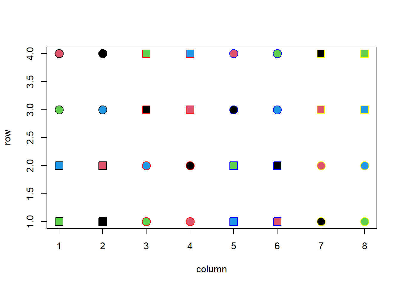
We can also have an schematic representation of the experiment by assigning the row and column columns to the x and y axes of a plot, and using the block and irrigation columns to color and shape the points, while the species is used to fill the points:
Analyze the randomization of the treatments. What kind of design is this?
Analyze this model with a standard linear model (ignore the species*irrigation interaction). What are the results?
Fit a linear mixed model to the data (same fixed effects as in point 2). Compare the results with the linear model.
Manually check the reported p-values for the coefficient irrigationNot_irrigated in the mixed model and the naive linear model (tip: this are the t-tests on the model coefficient, not the F tests on the predictors, we saw these t-test in earlier chapters).
Solution 5.1
We see that a block is composed of two columns and 4 rows (so 8 plots) and each block is divided into two halves, one with irrigation and one without (main plots). Within each main plot we have four sub-plots that are assigned the four species. So species is nested within irrigation, all blocks contains the 8 treatments and the assignment of irrigation and species appear to be random (at least there are no clear biases from the diagram). We would therefore concluded that this is a split-plot randomized complete block design.
We can analyze the data with a standard linear model. If we ignore the interaction term this leads to:
lm1 <-lm(yield ~ irrigation + species + block, data = dat)summary(lm1)
Call:
lm(formula = yield ~ irrigation + species + block, data = dat)

Residuals:
    Min      1Q  Median      3Q     Max
-1.8656 -0.2706  0.1250  0.3131  1.5006

Coefficients:
                        Estimate Std. Error t value Pr(>|t|)
(Intercept)               4.3769     0.3760  11.640 2.34e-11 ***
irrigationNot_irrigated  -1.3338     0.2659  -5.016 3.99e-05 ***
speciesGa                 2.2800     0.3760   6.064 2.92e-06 ***
speciesnn                 4.5525     0.3760  12.107 1.04e-11 ***
speciesSm                 2.9875     0.3760   7.945 3.56e-08 ***
blockblock2              -0.7362     0.3760  -1.958   0.0620 .
blockblock3              -1.2575     0.3760  -3.344   0.0027 **
blockblock4              -0.4562     0.3760  -1.213   0.2368
---
Signif. codes:  0 '***' 0.001 '**' 0.01 '*' 0.05 '.' 0.1 ' ' 1

Residual standard error: 0.752 on 24 degrees of freedom
Multiple R-squared:  0.8872,    Adjusted R-squared:  0.8544
F-statistic: 26.98 on 7 and 24 DF,  p-value: 6.752e-10
anova(lm1)
Analysis of Variance Table

Response: yield
           Df Sum Sq Mean Sq F value    Pr(>F)
irrigation  1 14.231 14.2311 25.1627 3.989e-05 ***
species     3 85.926 28.6419 50.6432 1.565e-10 ***
block       3  6.647  2.2158  3.9178   0.02076 *
Residuals  24 13.574  0.5656
---
Signif. codes:  0 '***' 0.001 '**' 0.01 '*' 0.05 '.' 0.1 ' ' 1
The results show that the main effects of irrigation and species are significant. Note however that this ignores the nested structure of the split plot design, which leads to a large underestimation of standard errors and p-values.
We can fit a linear mixed model to the data. We will include the random effects for the blocks and the nested structure of the species within irrigation:
library(lme4)
Loading required package: Matrix
library(lmerTest)
Attaching package: 'lmerTest'
The following object is masked from 'package:lme4':

    lmer
The following object is masked from 'package:stats':

    step
lmm1 <-lmer(yield ~ irrigation + species + (1|block/irrigation), data = dat)summary(lmm1, ddf="Kenward-Roger")
Linear mixed model fit by REML. t-tests use Kenward-Roger's method [
lmerModLmerTest]
Formula: yield ~ irrigation + species + (1 | block/irrigation)
   Data: dat

REML criterion at convergence: 73

Scaled residuals:
     Min       1Q   Median       3Q      Max
-2.39536 -0.28200 -0.03744  0.60781  1.53040

Random effects:
 Groups           Name        Variance Std.Dev.
 irrigation:block (Intercept) 0.26732  0.5170
 block            (Intercept) 0.08932  0.2989
 Residual                     0.43190  0.6572
Number of obs: 32, groups:  irrigation:block, 8; block, 4

Fixed effects:
                        Estimate Std. Error      df t value Pr(>|t|)
(Intercept)               3.7644     0.3958 10.1824   9.511 2.19e-06 ***
irrigationNot_irrigated  -1.3337     0.4332  3.0000  -3.079   0.0542 .
speciesGa                 2.2800     0.3286 21.0000   6.939 7.45e-07 ***
speciesnn                 4.5525     0.3286 21.0000  13.854 4.93e-12 ***
speciesSm                 2.9875     0.3286 21.0000   9.092 9.99e-09 ***
---
Signif. codes:  0 '***' 0.001 '**' 0.01 '*' 0.05 '.' 0.1 ' ' 1

Correlation of Fixed Effects:
            (Intr) irrgN_ specsG spcsnn
irrgtnNt_rr -0.547
speciesGa   -0.415  0.000
speciesnn   -0.415  0.000  0.500
speciesSm   -0.415  0.000  0.500  0.500
anova(lmm1, ddf="Kenward-Roger")
Type III Analysis of Variance Table with Kenward-Roger's method
           Sum Sq Mean Sq NumDF DenDF F value    Pr(>F)
irrigation  4.094  4.0945     1     3   9.480   0.05418 .
species    85.926 28.6419     3    21  66.315 7.035e-11 ***
---
Signif. codes:  0 '***' 0.001 '**' 0.01 '*' 0.05 '.' 0.1 ' ' 1
We can see that the big difference is the fact that the degrees of freedom in the denominator of the F test for irrigation is only 3 (4 blocks - 1) instead of the 24 used for the naive linear models (we saw something similar with the frogs in buckets in the previous lecture). This has a big impact on the significance of these effect. The sums of squares are also different for irrigation. This illustrates the importance of taking into account the structure of the experiment when analyzing the data as otherwise we may overestimate our statistical power and declare effects to be significant when they are not.
We can manually check the p-value for the coefficient irrigationNot_irrigated by taking the t-values reported from summary on each model (see above) and using the corresponding “residual” degrees of freedom (this is equivalent to the degrees of freedom in the denominator of the F test). For the linear and mixed models these degrees of freedom are 24 and 3 respectively. We the can calculate the p-values from the t distributions:
# For the linear model, extract t value and calculate p-valuetval <-coef(summary(lm1))["irrigationNot_irrigated", "t value"]2*pt(-abs(tval), df=24)
[1] 3.989202e-05
# For the mixed model, extract t value and calculate p-valuetval <-coef(summary(lmm1))["irrigationNot_irrigated", "t value"]2*pt(-abs(tval), df=3)
[1] 0.05418
5.2 Linear algebra of mixed effect models
The package lme4 does not have built-in functions to extract the individual covariance matrices that are used in the mixed effect model. We have written two functions that extract the covariance matrices for the random effects and the full covariance matrix as shown in the lecture:
# Covariance matrix that combines random effects and residual (V = ZGZ^t + R)getV <-function(model) { Lamda<-getME(model,"Lambda") ##matrix with scaling factor for random sd (relative to sigma) var.lamda <-t(Lamda)%*%Lamda ## scale for variance (sigma^2) Z <-getME(model,"Z") sigma2 <-sigma(model)^2## var.g<-sigma2*var.lamda var.random <- (Z %*% var.g %*%t(Z)) var.resid <- sigma2 *Diagonal(nrow(Z)) var.y <- var.random + var.residinvisible(var.y)}# Covariance matrix for random effects (G)getG <-function(model) { Lamda<-getME(model,"Lambda") ##matrix with scaling factor for random sd (relative to sigma) var.lamda <-t(Lamda)%*%Lamda ## scale for variance (sigma^2) sigma2 <-sigma(model)^2## var.g<-sigma2*var.lamdainvisible(var.g)}
We can then use these functions to extract the covariance matrices for the random effects and the full covariance matrix for the mixed effect model:
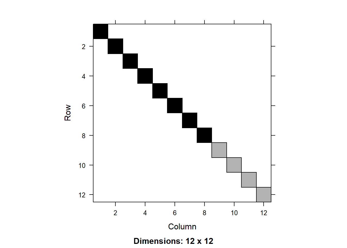
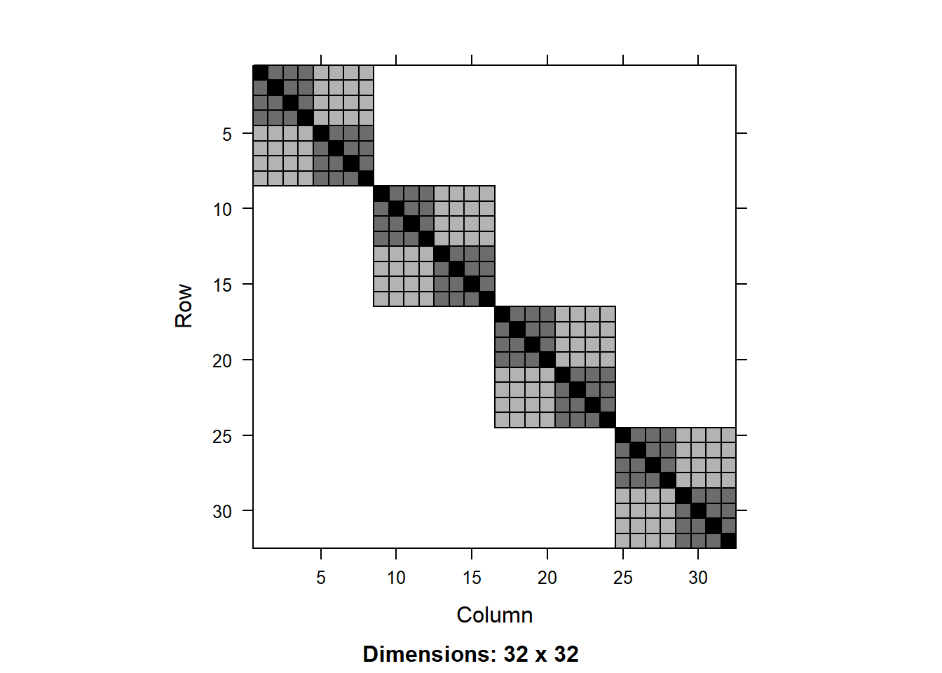
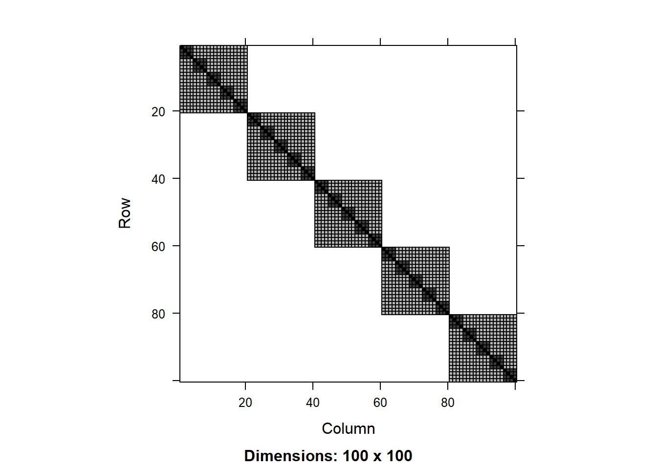
G <-getG(lmm1)V <-getV(lmm1)image(G)
image(V)
We can also extract the design matrix and the response vector from the model using the built-in function getME:
X <-getME(lmm1, "X")y <-getME(lmm1, "y")
Finally, we can extract the estimated fixed and random effects from the model directly ( useful for comparison):
Visualize the matrix V. Explain the structure of the matrices in relation to the experimental design.
Extract the different values being used in the matrix V and related them to the standard deviations/errors reported in the summary of the mixed model.
Estimate the coefficients of the fixed effects and their standard errors using the matrices and vectors extracted from the model. Compare the results with the output from the summary function.
Solution 5.2
We can visualize the matrices V and G using the image() function:
image(V)
As expected, we see a blocked matrix. A larger block is formed by the experimental block and include 8x8 elements in the matrix. Within each of those blocks we see two shades of color (units of 4x4) that correspond to the irrigation treatments (darker color indicate correlation of sub-plots within the same irrigation main plot). Finally, the diagonal represents the total variance of the data.
As usual, most of the values in the matrix are zeros, but there are three different values that are not zero (corresponding the three different shades of color in the visualization). We can extract these values as follows:
The values are 0.788 (diagonal), 0.357 (irrigation within block) and 0.089 (block).
Let’s see the variances that were estimated:
summary(lmm1)
Linear mixed model fit by REML. t-tests use Satterthwaite's method [
lmerModLmerTest]
Formula: yield ~ irrigation + species + (1 | block/irrigation)
   Data: dat

REML criterion at convergence: 73

Scaled residuals:
     Min       1Q   Median       3Q      Max
-2.39536 -0.28200 -0.03744  0.60781  1.53040

Random effects:
 Groups           Name        Variance Std.Dev.
 irrigation:block (Intercept) 0.26732  0.5170
 block            (Intercept) 0.08932  0.2989
 Residual                     0.43190  0.6572
Number of obs: 32, groups:  irrigation:block, 8; block, 4

Fixed effects:
                        Estimate Std. Error      df t value Pr(>|t|)
(Intercept)               3.7644     0.3958 10.1824   9.511 2.19e-06 ***
irrigationNot_irrigated  -1.3337     0.4332  3.0000  -3.079   0.0542 .
speciesGa                 2.2800     0.3286 21.0000   6.939 7.45e-07 ***
speciesnn                 4.5525     0.3286 21.0000  13.854 4.93e-12 ***
speciesSm                 2.9875     0.3286 21.0000   9.092 9.99e-09 ***
---
Signif. codes:  0 '***' 0.001 '**' 0.01 '*' 0.05 '.' 0.1 ' ' 1

Correlation of Fixed Effects:
            (Intr) irrgN_ specsG spcsnn
irrgtnNt_rr -0.547
speciesGa   -0.415  0.000
speciesnn   -0.415  0.000  0.500
speciesSm   -0.415  0.000  0.500  0.500
The variances are 0.432 (residual), 0.089 (block) and 0.267 (irrigation within block). The diagonal. The diagonal of the covariance matrix is the total variance of the data, so it should be equal to the sum of all variances:
0.432+0.089+0.267- V[1,1]
[1] -0.0005446907
Indeed that is the case (note that we only took 3 decimal digits hence the difference is not exactly zero).
The covariance within the irrigation main plots should be the sum of the variances associated to block and irrigation within block, so we can check that:
0.089+0.267- V[1,2]
[1] -0.0006399288
This is also the case. Finally, the covariance within a block (but across different irrigation plots) is just the variance of the block, so we can check that:
0.089- V[1,5]
[1] -0.0003232988
Of course this agreement is not a coincidence, the functions we used above to create V are also extracting the information from the fitted model (but in a way that is less transparent, so hopefully these manual checks help you understand the structure of the covariance matrix).
We can estimate the coefficients of the fixed effects with the familiar formula:
We can also compute the estimates of the random effects. This requires the covariance matrix of the random effects G (already extracted before) and the design matrix Z which we can extract from the model using the getME function:
Z <-getME(lmm1, "Z")
We also need the residual covariance matrix, which is just a diagonal matrix with the residual variance (or mean square error) which can computed as:
R <-diag(sigma(lmm1)^2, nrow =nrow(X))
We can then compute the estimates of the random effects using the formula:
u_hat <- G %*%t(Z) %*% V_inv %*% (y - X %*% beta)# The random effects for the irrigation main plotscbind(u_hat[1:8], ranef(lmm1)[[1]][[1]])
Note that u_hat contains all the random effects at the different levels (in this case there are two levels: block and irrigation within block). The ranef function returns the random effects for each level separately.
5.4 Simulating random effects and shrinkage
To test the ideas presented in the lecture, we are going to simulate some data from a population that can be described by a mixed effect model (this is the same synthetic data that was used in the slides). A simple model consists of a single random effect with an intercept. For example let’s assume we have 20 blocks with 5 observations per block:
b <-1:20r <-5data.sim <-data.frame(block =as.factor(rep(b, each = r)))
In many textbooks and tutorials/blogs, this type of problem is often introduced as students grades within schools, but we will leave this unspecified for now. The random effect model is specified by the following formula (make sure to include the ~ symbol at the start so that it becomes a formula):
ranef.form <-~ (1| block)
with the following parameters:
Fixef <-1000# Population averageVC_sd <-list(200, 800) # Standard deviation of random effect and residuals
We can simulate a possible sample from the response variable y given the model and parameters with the function simLMM from the designr package:
set.seed(123)library(designr) # Load the package. On first use, install with `install.packages("designr")data.sim$y<-simLMM(formula = ranef.form, data = data.sim, Fixef = Fixef, VC_sd = VC_sd)
Data simulation from a linear mixed-effects model (LMM)
Formula: gaussian ~ 1 + ( 1 | block )
empirical = FALSE
Random effects:
 Groups    Name          Std.Dev.  Corr
 block     (Intercept)   200.0
 Residual                800.0
Number of obs: 100, groups:  block, 20
Fixed effects:
(Intercept)
       1000
summary(data.sim)
     block          y
 1      : 5   Min.   :-727.7
 2      : 5   1st Qu.: 535.0
 3      : 5   Median : 979.8
 4      : 5   Mean   :1020.5
 5      : 5   3rd Qu.:1481.9
 6      : 5   Max.   :3107.2
 (Other):70
Exercise 5.3
Fit a linear model (with block as fixed effect andwithout intercept) and a linear mixed model to the simulated data where the intercept varies across blocks as a random effect.
Calculate the expected mean of the population from the linear model and the linear mixed model. Are they the same? How does it compare to the mean of the data?
Compare the residual variance of the two models. Are they the same?
Compare the estimated means of the blocks from the linear model and the linear mixed model. Are they the same?
Solution 5.3
We can fit a linear model to the data with lm:
lm2 <-lm(y ~ block -1, data = data.sim)summary(lm2)
lmm2 <-lmer(y ~ (1|block), data = data.sim)summary(lmm2)
Linear mixed model fit by REML. t-tests use Satterthwaite's method [
lmerModLmerTest]
Formula: y ~ (1 | block)
   Data: data.sim

REML criterion at convergence: 1590.9

Scaled residuals:
    Min      1Q  Median      3Q     Max
-2.1681 -0.5505 -0.1082  0.5882  2.6082

Random effects:
 Groups   Name        Variance Std.Dev.
 block    (Intercept)  81695   285.8
 Residual             472434   687.3
Number of obs: 100, groups:  block, 20

Fixed effects:
            Estimate Std. Error      df t value Pr(>|t|)
(Intercept)  1020.49      93.86   19.00   10.87 1.34e-09 ***
---
Signif. codes:  0 '***' 0.001 '**' 0.01 '*' 0.05 '.' 0.1 ' ' 1
We compute the mean of the population by averaging the block means in the linear model and in the data. For the linear mixed model, the intercept already represents the mean of the blocks:
c(lm2 =mean(coef(lm2)), lmm2 =fixef(lmm2), data =mean(data.sim$y))
             lm2 lmm2.(Intercept)             data
        1020.489         1020.489         1020.489
We can see that all the estimates are the same, that is comforting.
We can compare the residual variance of the two models:
c(lm2 =summary(lm2)$sigma, lmm2 =sigma(lmm2))
     lm2     lmm2
687.3386 687.3386
They are also the same.
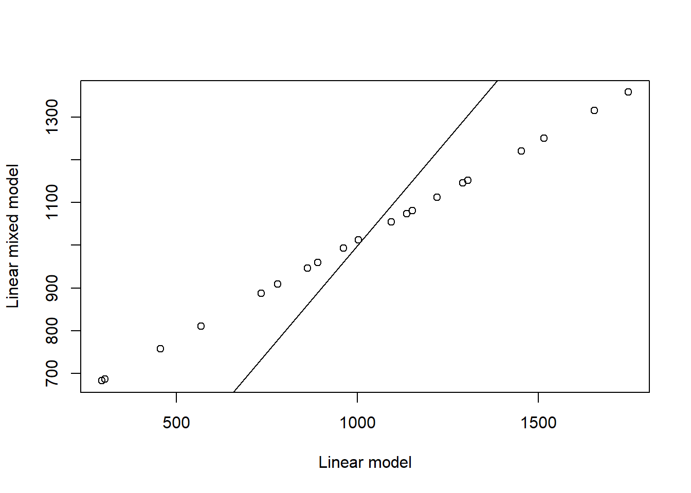
The mean of each block is given directly by the coefficients of the linear model (since we have no intercept) whereas in the linear mixed model it corresponds to the random effects plus the fixed effect:
This is the same figure as in the lecture, except that there we used the acronyms BLUP and BLUE. We can see that the range of values is smaller for the linear mixed model, this is also reflected on the variance:
c(lm2 =var(lm_means), lmm2 =var(lmm_means))
      lm2      lmm2
176182.19  37881.95
This is a neat example of the shrinkage effect of the linear mixed model. Be aware that the shrinkage effect does pull the estimates towards the population mean, so they will differ from the means derived direcrly from the data:
We can see that the means of the blocks are exactly the same in the linear model as when calculated directly from the data (and they should be!) but that is not the case for the linear mixed model because of shrinkage.
5.5 Interblock information
To illustrate how to retrieve interblock information, let’s simulate an extreme example of confounding between a quantitative variable and a grouping factor. We will add it to the previous block dataset:
We have added a variable rain that increases the response variable linearly. Since rain is perfectly correlated with the block variable, it creates a perfect confounding:
cor(data.sim$rain, as.numeric(data.sim$block))
[1] 1
Exercise 5.4
Fit a linear model and a linear mixed model to the simulated data, by adding rain as a fixed factor to the models fitted in the previous exercise.
Solution 5.4
We can fit the models as follows:
lm3 <-lm(y.rain ~ block + rain, data = data.sim)lmm3 <-lmer(y.rain ~ (1|block) + rain, data = data.sim)
Linear mixed model fit by REML. t-tests use Satterthwaite's method [
lmerModLmerTest]
Formula: y.rain ~ (1 | block) + rain
   Data: data.sim

REML criterion at convergence: 1583.3

Scaled residuals:
     Min       1Q   Median       3Q      Max
-2.15591 -0.51412 -0.09107  0.60804  2.61734

Random effects:
 Groups   Name        Variance Std.Dev.
 block    (Intercept)  89500   299.2
 Residual             472434   687.3
Number of obs: 100, groups:  block, 20

Fixed effects:
            Estimate Std. Error      df t value Pr(>|t|)
(Intercept)  1097.42     199.25   18.00   5.508 3.14e-05 ***
rain           42.67      16.63   18.00   2.566   0.0195 *
---
Signif. codes:  0 '***' 0.001 '**' 0.01 '*' 0.05 '.' 0.1 ' ' 1

Correlation of Fixed Effects:
     (Intr)
rain -0.877
We can see that the linear model is incapable of estimating the effect of rain because it has already captured the effect of each individual block. Note that the summary of the linear model mentions singularities at the top of the coefficients table. Remember that this has to do with the internal linear algebra of the model and suggests that the model has too many coefficients that cannot all be estimated. In the linear mixed model however, we do get an estimate of the effect of rain that is actually close to the theoretical value.
How is this possible? Well, in the linear model, the mean of each block is equal to the mean in the data (minus the effect of rain in the extended dataset), so the two predictors remain confounded. However, in the linear mixed model, the mean of each block can differ from the mean of the data because of shrinkage. This allows to break the perfect correlation.
5.6 Crossed vs nested random effects
Remember that random effects can be nested or not nested (i.e., crossed). To illustrate the difference between the two, let’s simulate a dataset with only random effects and fit the two types of models. We will create two random effects and a single intercept, similar to how we did it in the previous section:
# NUmber of levels for each random effect and repetitionsA <-1:10# First random effectB <-1:5# Second random effectr <-4# Number of repetitions per combination of random effects# Create all combinationsdata.sim <-expand.grid(A = A, B = B, rep =1:r)# Transform into factors and orderdata.sim$A <-factor(data.sim$A)data.sim$B <-factor(data.sim$B)data.sim$rep <-factor(data.sim$rep)indices <-with(data.sim, order(A, B, rep))data.sim <- data.sim[indices,]
Let’s specify the model as crossed random effects
ranef.form <-~ (1|A) + (1|B)
with the following parameters:
Fixef <-1000# Population averageVC_sd <-list(800, 400, 200) # Standard deviation of random effects (A and B) and residuals
Data simulation from a linear mixed-effects model (LMM)
Formula: gaussian ~ 1 + ( 1 | A ) + ( 1 | B )
empirical = FALSE
Random effects:
 Groups    Name          Std.Dev.  Corr
 A         (Intercept)   800.0
 B         (Intercept)   400.0
 Residual                200.0
Number of obs: 200, groups:  A, 10; B, 5
Fixed effects:
(Intercept)
       1000
and fit two linear mixed models, one with nested random effects (B within A) and one with crossed random effects:
lmm_nested <-lmer(y ~ (1|A/B), data = data.sim) # Nested random effects (wrong model)lmm_crossed <-lmer(y ~ (1|A) + (1|B), data = data.sim) # Cross random effects (correct model)
Exercise 5.5
Compare the estimates of the random effects in the two models. What do you see and can you explain it?
Extract the covariance matrix of each model (use getV(), visualize them and explain the differences.)
Solution 5.5
Let’s print the summaries of the two models:
summary(lmm_nested)
Linear mixed model fit by REML. t-tests use Satterthwaite's method [
lmerModLmerTest]
Formula: y ~ (1 | A/B)
   Data: data.sim

REML criterion at convergence: 2801.1

Scaled residuals:
     Min       1Q   Median       3Q      Max
-2.06117 -0.57270 -0.08432  0.60307  2.48154

Random effects:
 Groups   Name        Variance Std.Dev.
 B:A      (Intercept)  70841   266.2
 A        (Intercept) 541770   736.1
 Residual              37031   192.4
Number of obs: 200, groups:  B:A, 50; A, 10

Fixed effects:
            Estimate Std. Error     df t value Pr(>|t|)
(Intercept)   1182.1      236.2    9.0   5.005 0.000734 ***
---
Signif. codes:  0 '***' 0.001 '**' 0.01 '*' 0.05 '.' 0.1 ' ' 1
summary(lmm_crossed)
Linear mixed model fit by REML. t-tests use Satterthwaite's method [
lmerModLmerTest]
Formula: y ~ (1 | A) + (1 | B)
   Data: data.sim

REML criterion at convergence: 2727.2

Scaled residuals:
    Min      1Q  Median      3Q     Max
-2.3460 -0.6646 -0.0463  0.5909  3.2419

Random effects:
 Groups   Name        Variance Std.Dev.
 A        (Intercept) 555985   745.6
 B        (Intercept)  72012   268.3
 Residual              36046   189.9
Number of obs: 200, groups:  A, 10; B, 5

Fixed effects:
            Estimate Std. Error      df t value Pr(>|t|)
(Intercept)  1182.06     264.92   12.35   4.462 0.000725 ***
---
Signif. codes:  0 '***' 0.001 '**' 0.01 '*' 0.05 '.' 0.1 ' ' 1
For the nested models we see two terms for the random effects, one for A and one for A:B. The latter reflects the random effects for B within A. For the crossed random effects we see two terms for the random effects, one for A and one for B. Note that the actual variances associated with the random effects and the residuals are different but similar between both models. The estimate of the intercept is the same in both models but not the standard error. Overall, not a huge difference.
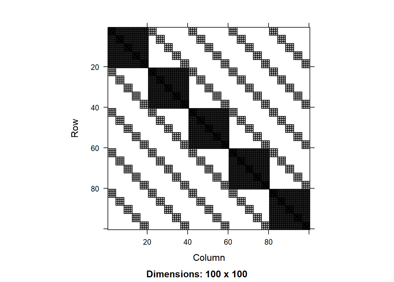
We can extract the covariance matrices of the two models:
We can see that for the crossed random effects the covariance matrix has multiple diagonals of blocks of 4x4 elements. This represents the correlation among observations that share the same B. In addition, we see larger blocks of 20x20 centered around the main diagonal that represent the correlation among observations that share the same A. For the nested random effects, we see the usual patter of nested blocks around the main diagonal.