In this section we will explore the effects of heterogeneous variance in observations on our statistical models. We will use a new dataset on nutrient uptake by crops across different fertilization trials:
    state             district          community               uN
 Length:692         Length:692         Length:692         Min.   :  1.933
 Class :character   Class :character   Class :character   1st Qu.: 37.670
 Mode  :character   Mode  :character   Mode  :character   Median : 64.420
                                                          Mean   : 70.533
                                                          3rd Qu.: 97.172
                                                          Max.   :233.042
       uP                uK          treatment            tot.biom
 Min.   : 0.1486   Min.   :  2.73   Length:692         Min.   :  378.7
 1st Qu.: 5.5811   1st Qu.: 37.76   Class :character   1st Qu.: 5087.0
 Median : 9.9041   Median : 62.00   Mode  :character   Median : 8033.0
 Mean   :11.2157   Mean   : 70.08                      Mean   : 7974.1
 3rd Qu.:15.2280   3rd Qu.: 92.50                      3rd Qu.:10619.1
 Max.   :42.8958   Max.   :351.44                      Max.   :20418.4
      soil
 Min.   :  1.00
 1st Qu.: 47.00
 Median : 93.50
 Mean   : 88.49
 3rd Qu.:129.00
 Max.   :165.00
As usual, let’s make sure all the relevant variables are encoded as factors and check for balance in the design:
As with previous exercises, the data is not balanced across the combination of factors.
Exercise 7.1
Fit a linear mixed model of P uptake (uP) with treatment as a fixed effect and soil as random effect (there are no slopes, so only vary the intercept across levels of soil).
Perform an anova on the model to check if the fixed effect is significant.
Plot the residuals of the model against the fitted values. What do you see?
Simulate data from the same structure of the model (just use simulate() on the model object) and fit the same model on that generated data. Plot the residuals of the new model and compared to the residuals of the original model.
Solution 7.1
We fit a linear mixed model using lmer():
library(lme4)
Loading required package: Matrix
library(lmerTest)
Attaching package: 'lmerTest'
The following object is masked from 'package:lme4':

    lmer
The following object is masked from 'package:stats':

    step
lmm1 <-lmer(uP ~ treatment + (1|soil), data = trial.dat)summary(lmm1)
Linear mixed model fit by REML. t-tests use Satterthwaite's method [
lmerModLmerTest]
Formula: uP ~ treatment + (1 | soil)
   Data: trial.dat

REML criterion at convergence: 4221.3

Scaled residuals:
    Min      1Q  Median      3Q     Max
-2.5615 -0.5885 -0.1043  0.4983  4.5136

Random effects:
 Groups   Name        Variance Std.Dev.
 soil     (Intercept) 26.37    5.135
 Residual             16.27    4.034
Number of obs: 692, groups:  soil, 165

Fixed effects:
             Estimate Std. Error       df t value Pr(>|t|)
(Intercept)    6.7778     0.5338 346.7241  12.696  < 2e-16 ***
treatmentNK    2.7042     0.4981 532.3110   5.429 8.63e-08 ***
treatmentNP    7.5706     0.4937 533.1901  15.336  < 2e-16 ***
treatmentNPK   9.3828     0.4983 532.1496  18.830  < 2e-16 ***
treatmentPK    2.9097     0.4933 529.1447   5.899 6.53e-09 ***
---
Signif. codes:  0 '***' 0.001 '**' 0.01 '*' 0.05 '.' 0.1 ' ' 1

Correlation of Fixed Effects:
            (Intr) trtmNK trtmNP trtNPK
treatmentNK -0.466
treatmentNP -0.472  0.507
treatmntNPK -0.466  0.504  0.511
treatmentPK -0.466  0.502  0.503  0.501
The summary looks ok, no convergence issues or warnings.
We perform an ANOVA on the model:
anova(lmm1, ddf ="Kenward-Roger")
Type III Analysis of Variance Table with Kenward-Roger's method
          Sum Sq Mean Sq NumDF  DenDF F value    Pr(>F)
treatment 7769.8  1942.5     4 533.29  119.37 < 2.2e-16 ***
---
Signif. codes:  0 '***' 0.001 '**' 0.01 '*' 0.05 '.' 0.1 ' ' 1
The treatment is clearly significant.
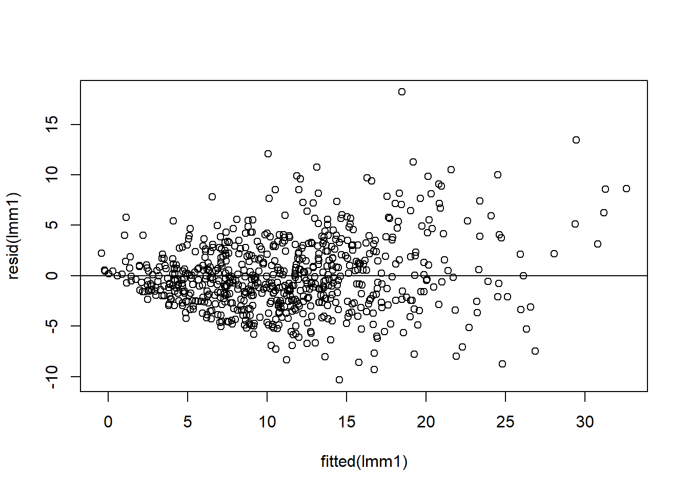
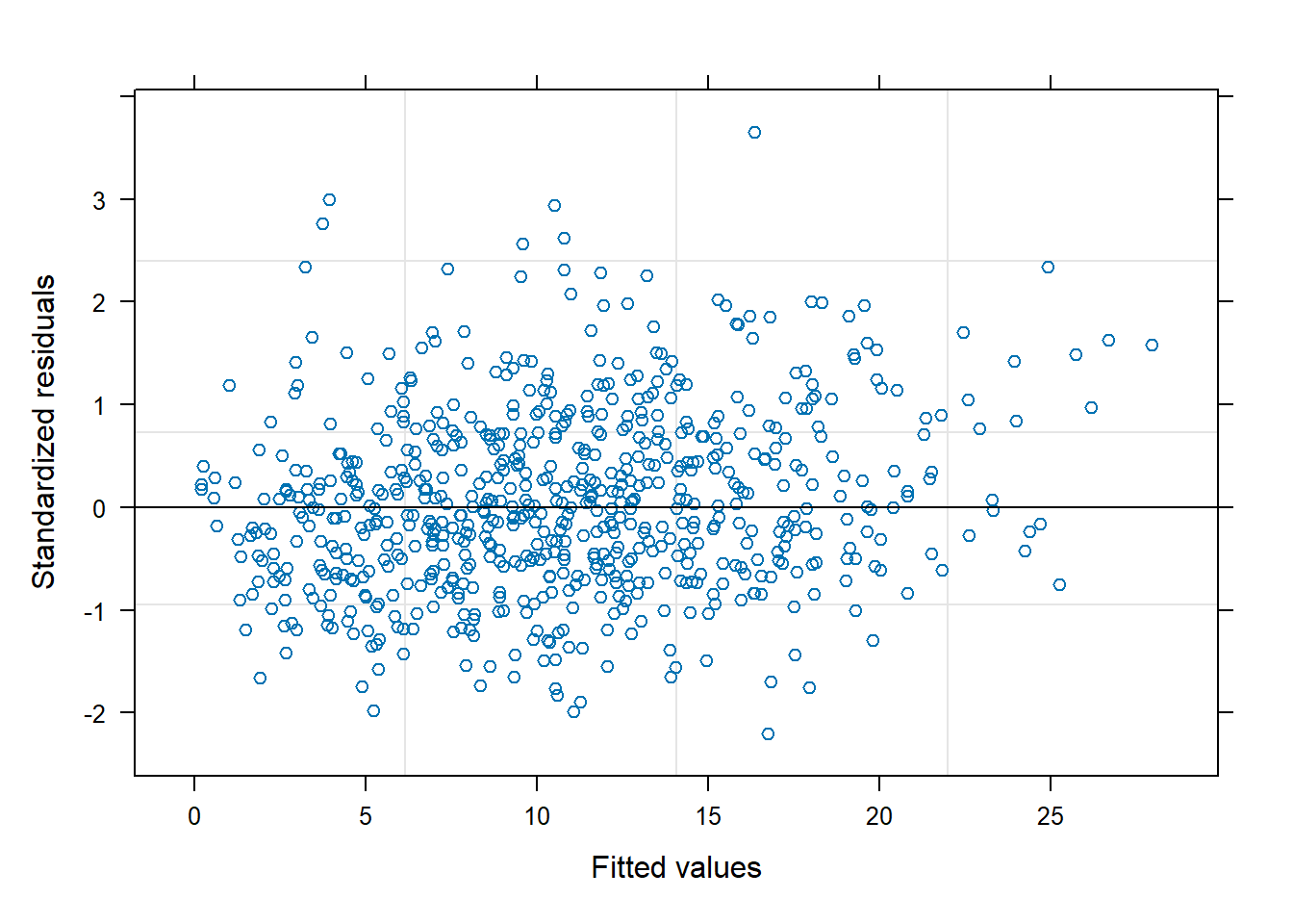
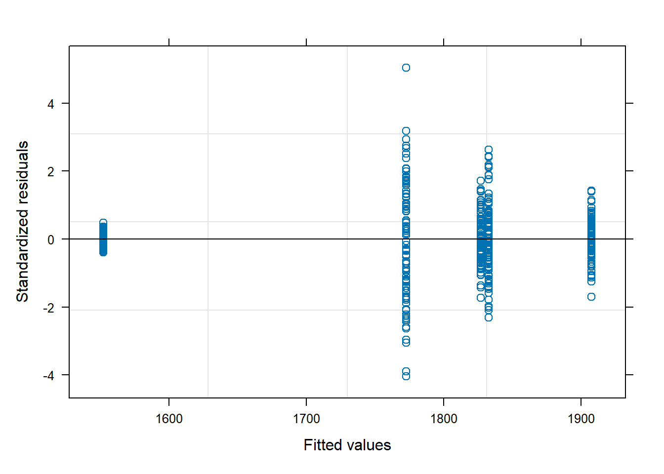
We plot the residuals of the model against the fitted values:
plot(fitted(lmm1), resid(lmm1))abline(h =0)
We see the fan effect in the residuals, which is a clear sign of heteroscedasticity. The variance of the observations is larger for larger values of P uptake.
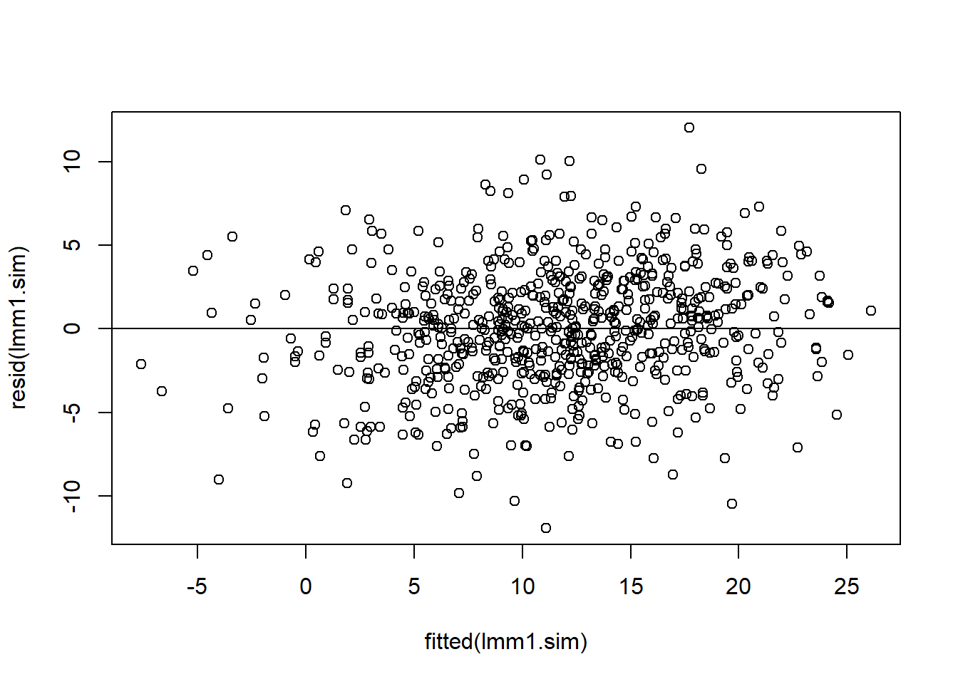
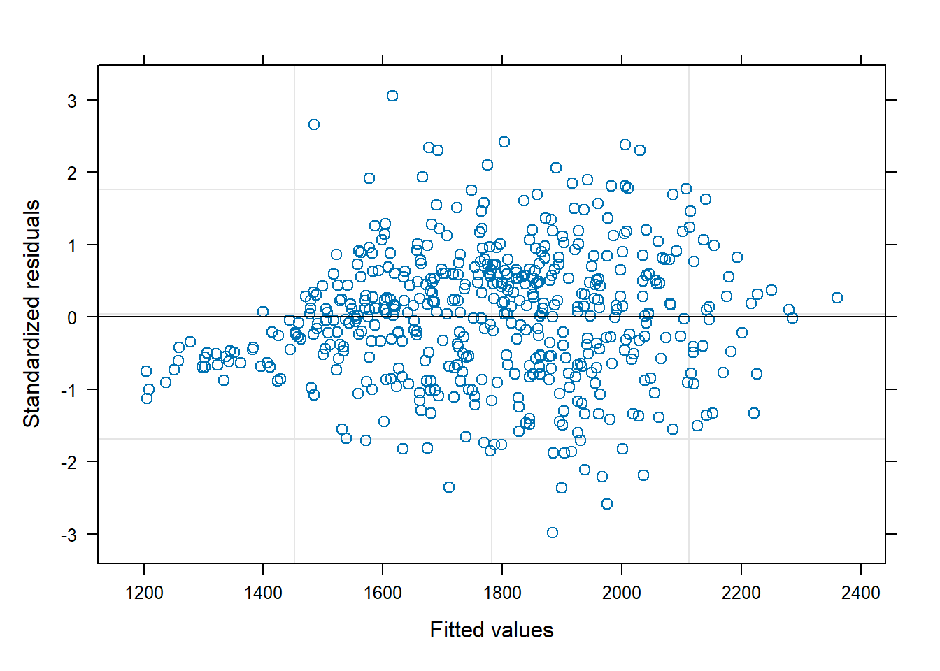
We simulate data from the same structure of the model and fit the same model on that generated data:
No we cannot see any fan effect in the residuals, the variance is constant across the fitted values. Of course, the data was simulated from a model that assumes a constant variance. This reinforces the idea that the original model was not capturing the true behavior of the data as it cannot reproduce similar patterns.
7.2 The package nlme and variance models
As shown in the lecture, we can model the variance of the observations as a function of predictors in order to account for heteroscedasticity. Unfortunately, the package lme4 does not support this feature. Instead, we can use the package nlme to fit a linear mixed model with a variance structure.
Let’s try three different models that differ in the variance structure. First, a model equivalent to the one fitted in the exercises (constant variance):
library(nlme)
Attaching package: 'nlme'
The following object is masked from 'package:lme4':

    lmList
lmme1.0<-lme(uP ~ treatment, random =~1|soil, data = trial.dat)
By default, lme() fits a model with constant variance. Note that the syntax is slightly different from lmer() (the random effect is assigned to a different argument of the function), but the idea is the same. Let’s fit a second model that assuments the variance increases as a power function of the total biomass (tot.biom):
lmme1.1<-lme(uP ~ treatment, random =~1|soil, weights =varPower(form =~tot.biom),data = trial.dat)
We assign the variance structure to the weights argument of the function and use a formula to specify which predictor to use. Finally, let’s fit a model that assumes the variance increases as a power function of the fitted values (the default form for varPower()):
lmme1.2<-lme(uP ~ treatment, random =~1|soil, weights =varPower(),data = trial.dat)
Notice that the output is really the same as in the lme4 package. The model that performs the best (according to the log-likelihood ratio test) is the one with the power function of fitted values.
If we now plot the residuals vs fitted values we should no longer see a fan effect in the models with heterogeneous variance. That is because these residuals are already corrected for the variance structure assumed in the model.
plot(lmme1.0,cex.lab=0.5)
plot(lmme1.1,cex.lab=0.5)
plot(lmme1.2,cex.lab=0.5)
When using lme() we can also extract the variance components of the model using VarCorr():
Just like for lmer() models, we can extract the covariance matrix of the models. The functions are somewhat different though and are stored in the package nlraa. Let’s extract the combined covariance matrix of the first model as well as the matrices for the residuals and random effects:
library(nlraa)# Full model covariance matrixV0 <-Matrix(var_cov(lmme1.0, type ="all", aug=T), sparse =TRUE)# Residual covariance matrixR0 <-Matrix(var_cov(lmme1.0, type ="residual", aug=T), sparse =TRUE)# Random effects covariance matrixG0 <-Matrix(var_cov(lmme1.0, type ="random", aug=T), sparse =TRUE)
Exercise 7.2
Extract the covariance matrices for the models lmme1.1 and lmme1.2 and compare them with the matrices extracted for the model lmme1.0. What do you see?
Same as 1 but for the variance components themselves (i.e., the values from VarCorr()).
What is the value assigned to the power function of the variance in the models with heterogeneous variance?
Using the full model covariance matrix, estimate the fixed effects and their standard errors for the model lmme1.1
Solution 7.2
We can extract the matrices using analogous code as in the above:
V0.1<-Matrix(var_cov(lmme1.1, type ="all", aug=T), sparse =TRUE)R0.1<-Matrix(var_cov(lmme1.1, type ="residual", aug=T), sparse =TRUE)G0.1<-Matrix(var_cov(lmme1.1, type ="random", aug=T), sparse =TRUE)V0.2<-Matrix(var_cov(lmme1.2, type ="all", aug=T), sparse =TRUE)R0.2<-Matrix(var_cov(lmme1.2, type ="residual", aug=T), sparse =TRUE)G0.2<-Matrix(var_cov(lmme1.2, type ="random", aug=T), sparse =TRUE)
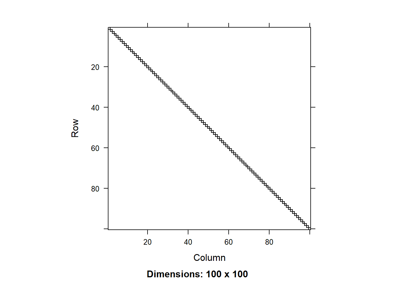
We can compare the matrices using the image() function. Let’s do that for the residual matrix first:
image(round(R0[1:100,1:100],3))
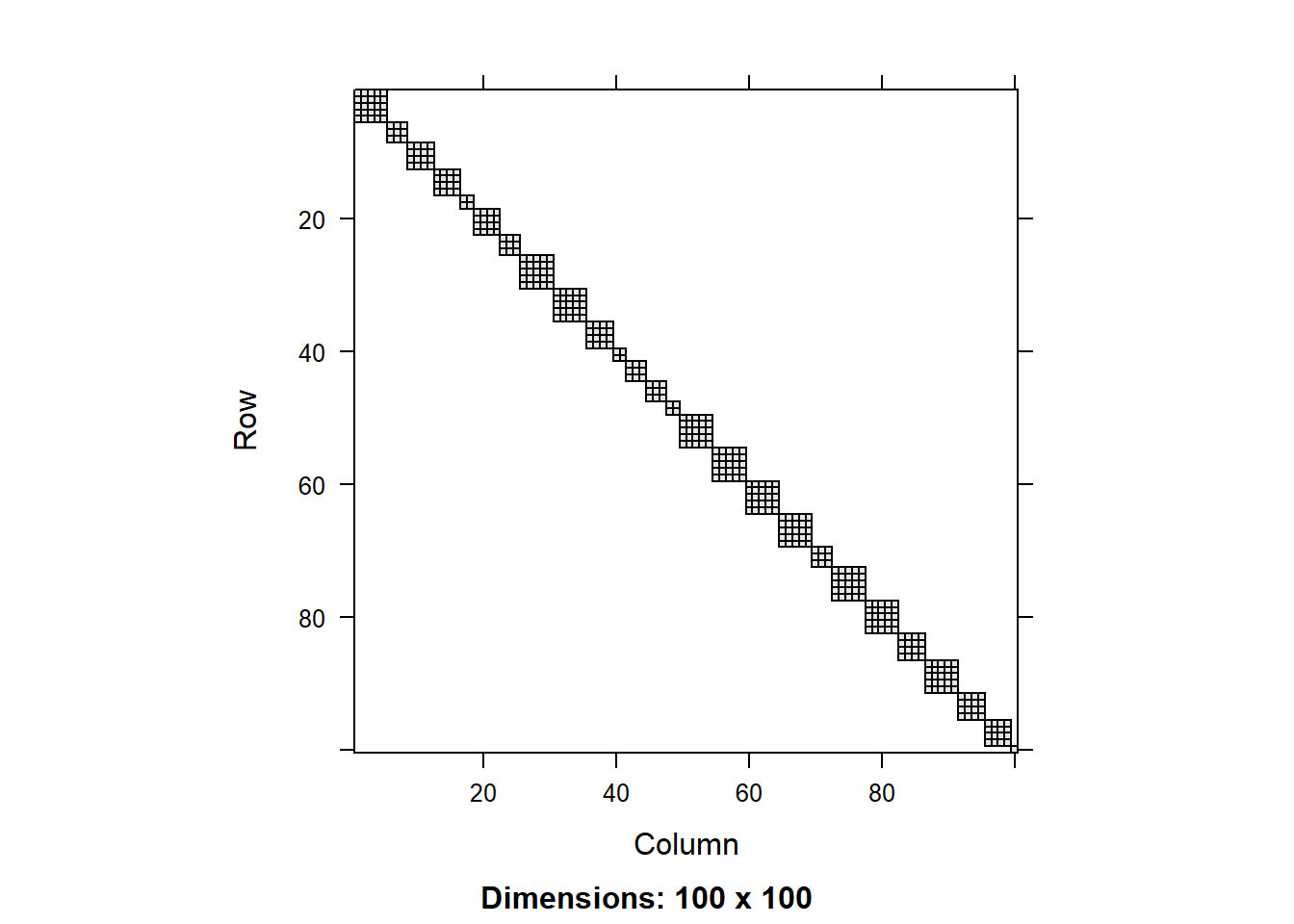
image(round(R0.1[1:100,1:100],3))
image(round(R0.2[1:100,1:100],3))
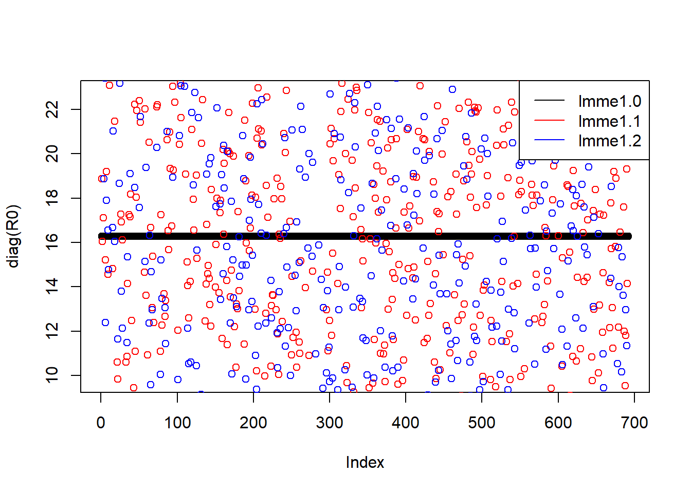
We can see that the residual covariance matrix has different values along the diagonal for the two models with heterogeneous variance. We can also plot the diagonal values as a scatter plot:
We can see that tjhe variance component for the random effect is similar across the models, but there is a significant difference in the residual variance. That is because the models with heterogeneous variance are able to explain a big part of the the variance in the data using the fitted values of total biomass, so this residual variance is smaller.
The value assigned to the power function of the variance in the models with heterogeneous variance can be read from the summary():
summary(lmme1.1)
Linear mixed-effects model fit by REML
  Data: trial.dat
       AIC      BIC    logLik
  4173.012 4209.271 -2078.506

Random effects:
 Formula: ~1 | soil
        (Intercept)   Residual
StdDev:    4.874494 0.04828493

Variance function:
 Structure: Power of variance covariate
 Formula: ~tot.biom
 Parameter estimates:
   power
0.494853
Fixed effects:  uP ~ treatment
                Value Std.Error  DF   t-value p-value
(Intercept)  6.532244 0.4596008 523 14.212865       0
treatmentNK  1.930125 0.3780541 523  5.105421       0
treatmentNP  6.847729 0.4423666 523 15.479760       0
treatmentNPK 8.429219 0.4557619 523 18.494786       0
treatmentPK  2.131140 0.3570543 523  5.968671       0
 Correlation:
             (Intr) trtmNK trtmNP trtNPK
treatmentNK  -0.345
treatmentNP  -0.316  0.369
treatmentNPK -0.300  0.352  0.318
treatmentPK  -0.357  0.425  0.368  0.356

Standardized Within-Group Residuals:
        Min          Q1         Med          Q3         Max
-3.02683264 -0.46173928  0.05908251  0.59778276  3.63042929

Number of Observations: 692
Number of Groups: 165
summary(lmme1.2)
Linear mixed-effects model fit by REML
  Data: trial.dat
       AIC      BIC    logLik
  4094.447 4130.706 -2039.224

Random effects:
 Formula: ~1 | soil
        (Intercept)  Residual
StdDev:    4.492757 0.6457648

Variance function:
 Structure: Power of variance covariate
 Formula: ~fitted(.)
 Parameter estimates:
    power
0.7708593
Fixed effects:  uP ~ treatment
                Value Std.Error  DF   t-value p-value
(Intercept)  6.693895 0.3999973 523 16.734852       0
treatmentNK  1.653936 0.2517275 523  6.570344       0
treatmentNP  7.311278 0.4163718 523 17.559496       0
treatmentNPK 9.088335 0.4633088 523 19.616149       0
treatmentPK  2.429505 0.2837447 523  8.562294       0
 Correlation:
             (Intr) trtmNK trtmNP trtNPK
treatmentNK  -0.221
treatmentNP  -0.182  0.200
treatmentNPK -0.164  0.184  0.145
treatmentPK  -0.218  0.262  0.191  0.179

Standardized Within-Group Residuals:
        Min          Q1         Med          Q3         Max
-2.20678437 -0.56438234 -0.01086811  0.63396692  3.65497914

Number of Observations: 692
Number of Groups: 165
The values are reported under the header Variance function, between the variance the sections on random effects and fixed effects.
We can estimate the fixed effects and their standard errors using the full covariance matrix of the model using the usual formulae. First we extract the design matrix, the response variable and the inverse of the covariance matrix:
X <-model.matrix(lmme1.1, data = trial.dat)y <- trial.dat$uPV_inv <-solve(V0.1)
Now we can estimate the fixed effects and their standard errors:
Sometimes, the variance in the residuals is caused by the grouping structure of the data. That is, in some groups the variance is larger than in others. We can model this using the nlme package by specifying a variance structure that depends on factors. This is the special variance model varIdent().
To illustrate this effect we are going to simulate some data. Let’s assume measurements on different varieties of a crop. The variance in the observations will vary across different varieties and all mthe observations are nested within farms:
mu <-2000# overall meann.var <-5# number of varietiesn.farm <-100# number of farmsVariety <-factor(1: n.var) # varieties coded with numbersFarm <-factor(1: n.farm) # farms coded with numbers
We can generate the fixed and random effects from centered normal distributions:
set.seed(123)Farm.effect <-rnorm(n.farm, mean =0, sd =200) # random effect of farmsVariety.effect <-rnorm(n.var, mean =0, sd =500) # fixed effect of varieties
We can then generate the residual standard deviations for each variety:
sigma.err <-runif(n.var, min =10, max =3000) #uniform draw of variety specific sdnames(sigma.err) <- Variety
And generate the design matrix for the fixed and random effects (note that we remove the intercept term because we have generated the fixed and random effects with respect to a mean rather than an intercept):
Z <-model.matrix(~Farm -1, data = design)X <-model.matrix(~Variety -1, data = design)
Finally, we can generate the response variable using the familiar linear algebra but without include the observation error (residual) yet:
design$y.true <- mu + X%*%Variety.effect + Z%*%Farm.effect
And now we need to match the residual standar deviation to each row in the dataset to generated observed responses:
# link varieties to their error sdvm <-match(design$Variety, names(sigma.err))# Variety-specific errorerr.vec<-rnorm(nrow(design), mean =0, sd = sigma.err[vm])# Add to the true valuesdesign$y <- design$y.true + err.vec
Exercise 7.3
Fit a linear mixed model with Variety as a fixed effect and Farm as a random effect and assuming constant variance (use lme). Explore the summary and residual plot.
Correct for the heterogeneous variance across varieties using the varIdent() function as follows: weights = varIdent(form =~ 1| Variety). Compare the summary and residual plot to the previous model and check which of the two models is better.
Extract the different matrices and visualize them. Explain the differences between the matrices of the two models and how they relate to the structure of the simulated data.
Estimate the fixed effects and their standard errors for the model with heterogeneous variance.
Linear mixed-effects model fit by REML
  Data: design
      AIC      BIC    logLik
  8457.97 8487.402 -4221.985

Random effects:
 Formula: ~1 | Farm
        (Intercept) Residual
StdDev:   0.2867243 1196.392

Fixed effects:  y ~ Variety - 1
            Value Std.Error  DF  t-value p-value
Variety1 1832.725  119.6392 396 15.31877       0
Variety2 1827.109  119.6392 396 15.27182       0
Variety3 1907.503  119.6392 396 15.94379       0
Variety4 1772.476  119.6392 396 14.81518       0
Variety5 1552.145  119.6392 396 12.97354       0
 Correlation:
         Varty1 Varty2 Varty3 Varty4
Variety2 0
Variety3 0      0
Variety4 0      0      0
Variety5 0      0      0      0

Standardized Within-Group Residuals:
       Min         Q1        Med         Q3        Max
-4.0473009 -0.4490518  0.0205217  0.4514541  5.0513390

Number of Observations: 500
Number of Groups: 100
We can see that the variance associated with the random effect is very small (about 0.3) compared to the true value (around 200), whereas the residual variation does seem to be in the right order of magnitude. Also, the estimates for the different farms have the same standard error. The residual plot shows the large variation in the residual variance across the different varieties that is not being correct for.
plot(lmme1) # a quick way to plot the residuals vs fitted
To correct for heterogeneous variance across groups we can use the varIdent() function as follows:
lmme2 <-lme(y~ Variety -1, random =~1| Farm, data = design,weights =varIdent(form =~1| Variety))summary(lmme2)
Linear mixed-effects model fit by REML
  Data: design
       AIC      BIC    logLik
  8088.639 8134.889 -4033.319

Random effects:
 Formula: ~1 | Farm
        (Intercept) Residual
StdDev:    205.3746 1313.903

Variance function:
 Structure: Different standard deviations per stratum
 Formula: ~1 | Variety
 Parameter estimates:
         1          2          3          4          5
1.00000000 0.65257147 0.51241383 1.54259473 0.08286378
Fixed effects:  y ~ Variety - 1
            Value Std.Error  DF  t-value p-value
Variety1 1832.725 132.98574 396 13.78137       0
Variety2 1827.109  88.16692 396 20.72329       0
Variety3 1907.503  70.38897 396 27.09946       0
Variety4 1772.476 203.71990 396  8.70055       0
Variety5 1552.145  23.24489 396 66.77358       0
 Correlation:
         Varty1 Varty2 Varty3 Varty4
Variety2 0.036
Variety3 0.045  0.068
Variety4 0.016  0.023  0.029
Variety5 0.136  0.206  0.258  0.089

Standardized Within-Group Residuals:
       Min         Q1        Med         Q3        Max
-2.9863833 -0.6073607  0.0548796  0.5804781  3.0586814

Number of Observations: 500
Number of Groups: 100
The standard deviation of the random effect is now much closer to the true value. We can also see now that the standard errors for the estimates of the fixed effects vary across varieties. However, the residual plot still shows some heterogeneity (but now we also see a more uniform spread of fitted values).
plot(lmme2)
We can compare the two models using the log-likelihood ratio test:
anova(lmme1, lmme2)
      Model df      AIC      BIC    logLik   Test  L.Ratio p-value
lmme1     1  7 8457.970 8487.402 -4221.985
lmme2     2 11 8088.639 8134.889 -4033.319 1 vs 2 377.3314  <.0001
We can see that the model with the heterogeneous variance across groups is significantly better than the model with constant variance.
We can extract the matrices and visualize them with var_cov():
# Model with homogeneous varianceV0 <-Matrix(var_cov(lmme1, type="all", aug=T),sparse =TRUE)R0 <-Matrix(var_cov(lmme1, type="residual", aug=T),sparse =TRUE)G0 <-Matrix(var_cov(lmme1, type="random", aug=T),sparse =TRUE)# Model with heterogeneous varianceV1 <-Matrix(var_cov(lmme2, type="all", aug=T),sparse =TRUE)R1 <-Matrix(var_cov(lmme2, type="residual", aug=T),sparse =TRUE)G1 <-Matrix(var_cov(lmme2, type="random", aug=T),sparse =TRUE)
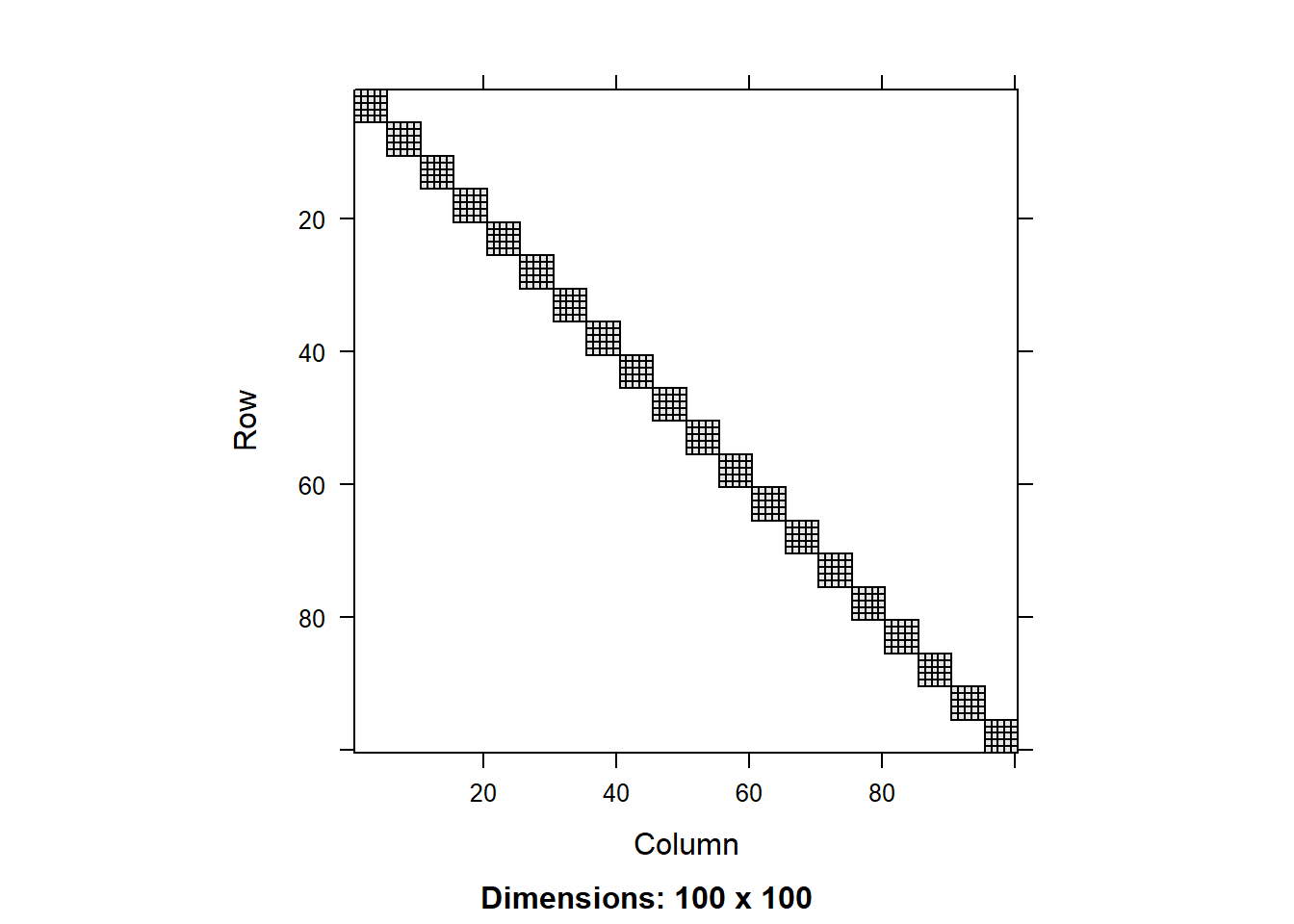
We can compare the matrices using the image() function. Let’s do that for the residual matrix first:
image(round(R0[1:100,1:100],3))
image(round(R1[1:100,1:100],3))
As expected, the second matrix shows different shades along the diagonal. Notice that there is a regular pattern, denoting the variances of the different varieties (the data is sorted by farm, so we are cycling through the varieties). Let’s look at the random effects covariance matrix:
image(round(G0[1:100,1:100],3))
image(round(G1[1:100,1:100],3))
The structure is identical, as the random effects are the same in both models. Finally, let’s look at the full covariance matrix:
image(round(V0[1:100,1:100],3))
image(round(V1[1:100,1:100],3))
As expected they differ in the diagonal only. We can extract the values of the variance components using the VarCorr() function:
As already discussed in the above the variance component for the random effect is quite off for the model with homogeneous variance.
We can estimate the fixed effects and their standard errors using the full covariance matrix of the model using the usual formulae. First we extract the design matrix, the response variable and the inverse of the covariance matrix:
X <-model.matrix(lmme2, data = design)y <- design$yV_inv <-solve(V1)
Now we can estimate the fixed effects and their standard errors: