dat <- read.csv("data/raw/Spacing and nitrogen_max225.csv", header = T)2 General linear model I
2.1 Linear model in R
2.1.1 A simple model (without interactions)
2.1.1.1 Fitting the model
Firstly, we need to load the data that we want to analyse. We have stored it as a comma-separated file:
We can get a summary of the contents of the data:
summary(dat) block plotnr Nitrogen Spacing
Min. :1.0 Min. : 1.000 Min. : 0.00 Length:24
1st Qu.:1.0 1st Qu.: 3.750 1st Qu.: 56.25 Class :character
Median :1.5 Median : 8.000 Median :112.50 Mode :character
Mean :1.5 Mean : 7.667 Mean :112.50
3rd Qu.:2.0 3rd Qu.:11.250 3rd Qu.:168.75
Max. :2.0 Max. :15.000 Max. :225.00
Yield treatment
Min. :27.17 Min. : 1.00
1st Qu.:36.69 1st Qu.: 3.75
Median :47.79 Median : 7.50
Mean :48.29 Mean : 7.50
3rd Qu.:57.92 3rd Qu.:11.25
Max. :69.20 Max. :14.00 Note that block and Spacing are encoded as numeric and character variables, respectively. However, we want to treat them as factor variables. This is necessary for fitting models in R and can also help with visualization. First, let’s check the unique values of block and Spacing:
unique(dat$block)[1] 1 2unique(dat$Spacing)[1] "less" "more" "recommended"We can confirm that the experiment has two blocks and there are three levels of spacing between plants. We can convert the variables to factors using the factor function:
dat$block <- factor(dat$block)
dat$Spacing <- factor(dat$Spacing, levels = c("less", "recommended", "more"))
Note that for Spacing we specify the argument levels. This can be used to indicate the order in which the levels should be treated. In this case, we have specified that the order is less, recommended, and more (i.e., from less to more spacing). If we do not specify the levels argument, R will order the levels in alphabetical order (so in this case that would be less, more, recommended, which does not make sense semantically).
A linear model is fit in R with lm(). We specify the model as a formula. The simplest model will include Spacing and block as fixed effects without interactions:
fit <- lm(Yield ~ block + Spacing, data = dat)2.1.1.2 Design matrix and coefficients
R will perform all the calculations and store the results in the object fit. We can get a summary of the model with the summary function:
summary(fit)
Call:
lm(formula = Yield ~ block + Spacing, data = dat)

Residuals:
    Min      1Q  Median      3Q     Max
-9.5629 -5.2039  0.1216  4.7532 13.1864

Coefficients:
                   Estimate Std. Error t value Pr(>|t|)
(Intercept)          61.406      2.905  21.141 3.74e-15 ***
block2              -19.592      2.905  -6.745 1.46e-06 ***
Spacingrecommended   -4.483      3.557  -1.260    0.222
Spacingmore          -5.465      3.557  -1.536    0.140
---
Signif. codes:  0 '***' 0.001 '**' 0.01 '*' 0.05 '.' 0.1 ' ' 1

Residual standard error: 7.115 on 20 degrees of freedom
Multiple R-squared:  0.7067,    Adjusted R-squared:  0.6627
F-statistic: 16.06 on 3 and 20 DF,  p-value: 1.495e-05
The summary provides the following information:
The original formula that was used to fit the model. This is helpful when fitting multiple models so that we can keep track of which model is which.
A summary of the residuals of the model (difference between the observed and predicted values). This is not very informative but later we will see how to extract the residuals from the model and use them for diagnostics.
The coefficients of the fixed effects of the model. In this simple model, we have an intercept (reference) that corresponds to the first level of
Spacingandblockand three coefficients that correspond to the fixed effect of the other levels ofSpacingandblock(i.e., the difference with respect to the reference level). Notice that R will name each coefficient with the name of the variable and the level. For example, the coefficientSpacingrecommendedcorresponds to the difference between therecommendedlevel ofSpacingand thelesslevel ofSpacing(forblock = 1).Per coefficient we have the estimate and associated standard error and the result of the t-test that compares each estimate to zero.
The last part of the summary includes the residual standard error (model error), the degrees of freedom and the \(R^2\) of the model. The final test (F-statistic) tests the null hypothesis that all coefficients of the model (except intercept) are zero.
We can also acces the design matrix with the model.matrix function:
X <- model.matrix(fit)
X
(Intercept) block2 Spacingrecommended Spacingmore
1 1 0 0 0
2 1 0 0 0
3 1 0 0 0
4 1 0 0 0
5 1 0 0 1
6 1 0 0 1
7 1 0 0 1
8 1 0 0 1
9 1 0 1 0
10 1 0 1 0
11 1 0 1 0
12 1 0 1 0
13 1 1 0 0
14 1 1 0 0
15 1 1 0 0
16 1 1 0 0
17 1 1 0 1
18 1 1 0 1
19 1 1 0 1
20 1 1 0 1
21 1 1 1 0
22 1 1 1 0
23 1 1 1 0
24 1 1 1 0
attr(,"assign")
[1] 0 1 2 2
attr(,"contrasts")
attr(,"contrasts")$block
[1] "contr.treatment"
attr(,"contrasts")$Spacing
[1] "contr.treatment"Remember that this matrix contains the values of all the coefficients of the model (columns) for every observation (rows). This matrix is created by R from the formula defining the model and the data.
For factors, R creates a matrix with 0s and 1s that indicates whether the observation belongs to a particular level of the factors, whereas for continuous variables, the matrix contains the values of the variable (but we do not have any in this model).
A special case is the intercept that always contains the value 1 to indicate that the intercept should be added to all observations. Remember that the first level of each factor is included in the intercept.
We can also access the estimates for the coefficients of the model with the coef function:
coef(fit) (Intercept) block2 Spacingrecommended Spacingmore
61.405678 -19.592116 -4.482659 -5.464717 We can recover the predictions of the model by multiplying the design matrix by the vector of coefficients as shown in the lecture. Let’s do it for the first observation:
y_hat <- sum(X[1,] * coef(fit))
y_hat
[1] 61.40568R will also do this operation for us when calling the predict or the fitted function:
y_hat2 <- predict(fit)[[1]]
y_hat3 <- fitted(fit)[[1]]
c(y_hat, y_hat2, y_hat3)
[1] 61.40568 61.40568 61.40568The difference between predict and fitted is that predict can be used to predict the response variable for new data (i.e., data that was not used to fit the model) whereas fitted can only be used to predict the response variable for the data that was used to fit the model.
2.1.1.3 Contrasts
The default contrasts in R are treatment contrasts where the coefficients of the model correspond to the differences between the levels of the factors and the reference level. This means that the order of levels of the factors is important as it determines which level is the reference level. This is the most common type of contrasts when analysing data from experiments, especially if you make sure that the first level of each factor is the control or reference level in the experiment (by default levels are ordered alphabetically, so you may need to adjust the order).
There are other types of contrasts that can be used to test different hypotheses from the same data. We can use the function glht from the package multcomp to define alternative contrasts and run tests on them.
Let’s imagine that we are interested in the following hypotheses:
\[ \begin{align*} H_0: \widehat{\mu}_{\text{less}} = \frac{\widehat{\mu}_{\text{more}} + \widehat{\mu}_{\text{rec}}}{2} \\ H_1: \widehat{\mu}_{\text{less}} \neq \frac{\widehat{\mu}_{\text{more}} + \widehat{\mu}_{\text{rec}}}{2} \end{align*} \]
This is a two-sided test where a new reference level is defined as the average of two of the existing levels. In order to build the contrast we need to rephrase the null hypothesis as a comparison to 0 and in terms of the coefficients of the model. That is:
\[ H_0: \widehat{\mu}_{\text{less}} - \frac{\widehat{\mu}_{\text{more}} + \widehat{\mu}_{\text{rec}}}{2} = 0, \]
Let’s check the coefficients of the model:
coef(fit) (Intercept) block2 Spacingrecommended Spacingmore
61.405678 -19.592116 -4.482659 -5.464717 and if we define the coefficients \(b_0\), \(b_2\) and \(b_3\) as the intercept (that includes Spacingless) and the two effects of spacing (Spacingrecommended and Spacingmore), then
\[ \begin{align*} \widehat{\mu}_{\text{less}} &&= b_0 \\ \widehat{\mu}_{\text{rec}} &&= b_0 + b_2 \\ \widehat{\mu}_{\text{more}} &&= b_0 + b_3 \end{align*} \]
Such that the null hypothesis can be written as:
\[ \begin{align*} b_0 - \frac{b_0 + b_3 + b_0 + b_2}{2} = 0. \\ b_0 - 0.5b_0 - 0.5b_2 - 0.5b_0 - 0.5b_3 = 0 \\ -0.5b_2 - 0.5b_3 = 0 \end{align*} \]
Notice that we skipped \(b_1\) because that corresponds to the effect of the second level of block (which is not relevant for this contrast). We can build the contrast matrix by specifying the coefficients of the model that we want to compare. Each column of the matrix represents a different coefficient of the model as returned by coef():
library(multcomp) # Install this the first time you use itLoading required package: mvtnormLoading required package: survivalLoading required package: TH.dataLoading required package: MASS
Attaching package: 'TH.data'The following object is masked from 'package:MASS':
geysercontrast <- matrix(c(0, 0, -0.5, -0.5), nrow = 1, ncol = 4)
contrast [,1] [,2] [,3] [,4]
[1,] 0 0 -0.5 -0.5To test this contrast we can use the glht function that takes the fitted model and the contrast matrix:
test_contrast <- glht(fit, contrast)
summary(test_contrast)
     Simultaneous Tests for General Linear Hypotheses

Fit: lm(formula = Yield ~ block + Spacing, data = dat)

Linear Hypotheses:
       Estimate Std. Error t value Pr(>|t|)
1 == 0    4.974      3.081   1.614    0.122
(Adjusted p values reported -- single-step method)
Let’s verify that the estimate of the difference is correct:
sum(coef(fit) * contrast)[1] 4.9736882.1.1.4 Uncertainty and significance
We can manually verify the t-test for the coefficient of Spacingrecommended (of course this is not necessary, but it is a good exercise to understand the output of the summary). Remember that the t statistic for a coefficient is calculated as the ratio between the estimate and its standard error:
t <-  -4.483/3.557
t
[1] -1.260332The t statistic is -1.261. We can calculate the p-value of the t-test using the pt function that calculates the cumulative density of the t-distribution:
2 * pt(t, df = 20)[1] 0.2220567Notice that we multiply the p-value by 2 because we are interested in a two-tailed test (i.e., whether the value of the coefficient different from zero regardless of whether it is positive or negative). Also, the t-distribution has 20 degrees of freedom (the residual degrees of freedom of the model). This calculations gives a total tail probability (p-value) that is much larger than 0.05, so we would not reject the null hypothesis that the coefficient is zero (i.e., we cannot claim an effect of fertilizer between the levels less and recommended).
The confidence intervals of the coefficients are not included in the summary of the model but can be calculated with the confint function:
confint(fit, level = 0.95) 2.5 % 97.5 %
(Intercept) 55.34672 67.464639
block2 -25.65108 -13.533154
Spacingrecommended -11.90334 2.938023
Spacingmore -12.88540 1.955964Note that the default value for level is 0.95, so we could have omitted it. Remember that the confidence interval comes from the t-distribution that we used before. Indeed, the 95% confidence interval for the coefficient of Spacingrecommended can be computed as follows:
E = qt(0.975, df = 20) # The 97.5% quantile of the t-distribution with 20 degrees of freedom
HW = 3.557 * E # Half-width of the confidence interval (standard error times quantile)
CI_lower = -4.483 - HW # Lower bound of the confidence interval (estimate minus half-width)
CI_upper = -4.483 + HW # Upper bound of the confidence interval (estimate plus half-width)
c(CI_lower, CI_upper)
[1] -11.902772 2.9367722.1.1.5 Marginal means
As described above, the coefficients of the model are the differences between the means at the different levels of the factors and the reference level. We may also be interested in calculating the means for each level (for a given factor or combination of factors) together with their uncertainty. These are called marginal means and we can compute them with the package emmeans. For example, to compute the marginal means and their uncertainty for each level of Spacing we can use the following code:
library(emmeans) # Install this the first time you use itWelcome to emmeans.
Caution: You lose important information if you filter this package's results.
See '? untidy'emmeans(fit, specs = "Spacing") # Specify the factor for which we want the marginal means Spacing emmean SE df lower.CL upper.CL
less 51.6 2.52 20 46.4 56.9
recommended 47.1 2.52 20 41.9 52.4
more 46.1 2.52 20 40.9 51.4
Results are averaged over the levels of: block
Confidence level used: 0.95 The function emmeans calculates the marginal means for each level of Spacing and the standard error and confidence intervals of these means. Notice that because we only specified Spacing in the specs argument, these are the marginal means for each level of Spacing regardless of the level of block. If we want to calculate the marginal means for each combination of Spacing and block we can specify both factors in the specs argument:
emmeans(fit, specs = c("Spacing", "block")) Spacing block emmean SE df lower.CL upper.CL
less 1 61.4 2.9 20 55.3 67.5
recommended 1 56.9 2.9 20 50.9 63.0
more 1 55.9 2.9 20 49.9 62.0
less 2 41.8 2.9 20 35.8 47.9
recommended 2 37.3 2.9 20 31.3 43.4
more 2 36.3 2.9 20 30.3 42.4
Confidence level used: 0.95 Notice that the standard errors are larger when we calculate the marginal means for each combination of Spacing and block than when we calculate the marginal means for each level of Spacing. This makes sense as we are using less data to calculate the means when we consider the combinations of Spacing and block than when we consider only Spacing. Note that in all cases the degrees of freedom reported are those of the model, so this is not affected by the number of groups for which we compute the means.
2.1.1.6 Diagnostic plots and assumptions
The quality of inferences made from the model depends on the assumptions of the model being met. When assumptions are related to the structure of the data, we can determine whether they are met before we fit the model by thinking about how the data was collected. However, other assumptions are related to the residuals of the model and can only be checked after the model is fitted.
A visual inspection of the residuals can help us to determine whether the assumptions of the model are met. For models fitted with lm we can generate a collection of diagnostic plots with the plot function. This will create 4 plots, so it good practice to create a matrix of panels first (with par(mfrow = c(2,2))):
par(mfrow = c(2,2)) # Create a 2x2 matrix of panels
plot(fit) # Generate the diagnostic plots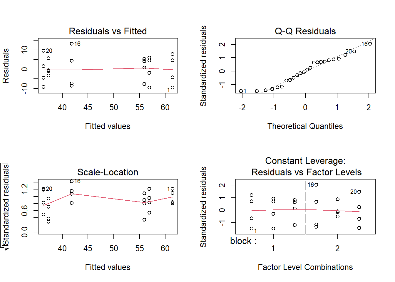
par(mfrow = c(1,1)) # Return to the default 1x1 panelIn the first panel (upper left) we have the residuals vs fitted values, both as individual pairs of values as well as a trend line. This plot is useful to detect non-linear relationships (i.e., the residuals should be randomly distributed around 0 in a symmetric fashion) as well as possible changes in variance.
Some of the data points are labelled with a number. These are observations that have been identified as possible outliers by the model and the number corresponds to the row in the data frame. Outliers correspond to absolute standardized residuals larger than 3. This does not mean that the observation is wrong (even if the model fits perfectly the data, there is a probability of 0.27% of an observation being declared an outlier, so if you have large enough data, you will eventually find some outliers).
The second panel (upper right) compares the quantiles of the residuals (standardized by the residual error) with the quantiles of a standard normal distribution (mean of zero and standard deviation of one), plus a 1:1 line. This plot is useful to detect departures from normality, especially for the larger residuals.
The third panel and fourth panel (lower left and right) are modifications of the first one and we will not cover them in detail here. You can check the documentation for more information (type ?plot.lm in the R console).
We can also run statistical tests to check the assumptions of the model. This is sometimes used to make decisions about whether to use a particular model. We do not necessarily endorse such protocols but nevertheless show how to perform the tests.
Firstly, we need to extract the residuals from the model:
res <- residuals(fit)We could then perform a Shapiro-Wilk test to check the normality of the residuals:
shapiro.test(res)
    Shapiro-Wilk normality test

data:  res
W = 0.94758, p-value = 0.24
The null hypothesis of the Shapiro-Wilk test is that the residuals are normally distributed and this result indicates that we would not reject this null hypothesis. We could also test if the variance of the residuals is constant across the different levels of the factors. This can be done with the Bartlett test:
bartlett.test(res, dat$Spacing)
    Bartlett test of homogeneity of variances

data:  res and dat$Spacing
Bartlett's K-squared = 1.5285, df = 2, p-value = 0.4657
The null hypothesis of the Bartlett test is that the variances of the residuals are equal across the different levels of the factor. In this case, we would not reject this null hypothesis.
Exercise 2.1
- Fit the same model as in section 2.1.1.1 to the data but remove the effect of
block. - Verify the t-value and p-value of the “Spacingrecommended” coefficient as shown above (i.e., using the
ptfunction and the formula for the t statistic). Calculate the confidence interval. What is the interpretation of this coefficient? - Calculate the fitted value for the 4th observation using the design matrix and compare to the output of
predict(do it for one observation). - Compute the marginal means for each level of
Spacingusing the coefficients and withemmeans. - Analyse the same contrast as in 2.1.1.3, but now using the model without
block. - Compare the results of the model with and without the effect of
blockand explain the difference. - Perform visual diagnostics on the model and run statistical tests on its assumptions.
Solution 2.1
- We fit the model without the effect of
block:
fit2 <- lm(Yield ~ Spacing, data = dat)
summary(fit2)
Call:
lm(formula = Yield ~ Spacing, data = dat)

Residuals:
     Min       1Q   Median       3Q      Max
-18.9753 -10.4367   0.2368  11.4226  17.5904

Coefficients:
                   Estimate Std. Error t value Pr(>|t|)
(Intercept)          51.610      4.442  11.617 1.32e-10 ***
Spacingrecommended   -4.483      6.283  -0.714    0.483
Spacingmore          -5.465      6.283  -0.870    0.394
---
Signif. codes:  0 '***' 0.001 '**' 0.01 '*' 0.05 '.' 0.1 ' ' 1

Residual standard error: 12.57 on 21 degrees of freedom
Multiple R-squared:  0.03934,   Adjusted R-squared:  -0.05215
F-statistic: 0.43 on 2 and 21 DF, p-value: 0.6561- We can verify the calculations for the coefficient of
Spacingrecommended. The t-statistic is calculated as:
t2 <- -4.483/6.283
t2
[1] -0.7135127The p-value of the t-test is:
2 * pt(t2, df = 21)[1] 0.4833835This coefficent represents the difference in means between the intercept (Spacing level “less”) and Spacing level “recommended”.
The confidence interval of the coefficient is:
confint(fit2, level = 0.95) 2.5 % 97.5 %
(Intercept) 42.37105 60.848191
Spacingrecommended -17.54797 8.582654
Spacingmore -18.53003 7.600595- We can calculate the fitted values from the design matrix and compare to the output of
predict. Let’s do it for the fourth observation:
X2 <- model.matrix(fit2)
y_hat <- sum(X2[4,] * coef(fit2))
y_hatp <- predict(fit2)[4]
c(y_hat, y_hatp)
4
51.60962 51.60962 - The marginal means are calculated as:
coef(fit2)[1] #mean "less"(Intercept)
51.60962 coef(fit2)[1]+coef(fit2)[2] #mean "recommended"(Intercept)
47.12696 coef(fit2)[1]+coef(fit2)[3] #mean "more"(Intercept)
46.1449 emmeans(fit2, specs = "Spacing") Spacing emmean SE df lower.CL upper.CL
less 51.6 4.44 21 42.4 60.8
recommended 47.1 4.44 21 37.9 56.4
more 46.1 4.44 21 36.9 55.4
Confidence level used: 0.95 - We can perform the contrast as before but now using the model without
block:
contrast2 <- matrix(c(0, -0.5, -0.5), nrow = 1, ncol = 3)
test_contrast2 <- glht(fit2, contrast2)
summary(test_contrast2)
     Simultaneous Tests for General Linear Hypotheses

Fit: lm(formula = Yield ~ Spacing, data = dat)

Linear Hypotheses:
       Estimate Std. Error t value Pr(>|t|)
1 == 0    4.974      5.441   0.914    0.371
(Adjusted p values reported -- single-step method)- Let’s compare the results of the two models by printing the summary of both models:
summary(fit)
Call:
lm(formula = Yield ~ block + Spacing, data = dat)

Residuals:
    Min      1Q  Median      3Q     Max
-9.5629 -5.2039  0.1216  4.7532 13.1864

Coefficients:
                   Estimate Std. Error t value Pr(>|t|)
(Intercept)          61.406      2.905  21.141 3.74e-15 ***
block2              -19.592      2.905  -6.745 1.46e-06 ***
Spacingrecommended   -4.483      3.557  -1.260    0.222
Spacingmore          -5.465      3.557  -1.536    0.140
---
Signif. codes:  0 '***' 0.001 '**' 0.01 '*' 0.05 '.' 0.1 ' ' 1

Residual standard error: 7.115 on 20 degrees of freedom
Multiple R-squared:  0.7067,    Adjusted R-squared:  0.6627
F-statistic: 16.06 on 3 and 20 DF, p-value: 1.495e-05summary(fit2)
Call:
lm(formula = Yield ~ Spacing, data = dat)

Residuals:
     Min       1Q   Median       3Q      Max
-18.9753 -10.4367   0.2368  11.4226  17.5904

Coefficients:
                   Estimate Std. Error t value Pr(>|t|)
(Intercept)          51.610      4.442  11.617 1.32e-10 ***
Spacingrecommended   -4.483      6.283  -0.714    0.483
Spacingmore          -5.465      6.283  -0.870    0.394
---
Signif. codes:  0 '***' 0.001 '**' 0.01 '*' 0.05 '.' 0.1 ' ' 1

Residual standard error: 12.57 on 21 degrees of freedom
Multiple R-squared:  0.03934,   Adjusted R-squared:  -0.05215
F-statistic:  0.43 on 2 and 21 DF,  p-value: 0.6561
We can see that the intercept of the model without block is different from the intercept of the model with block. This is because the intercept of the model with block is the mean of the first level of block and the first level of Spacing whereas the intercept of the model without block is just the mean of the first level of Spacing (pooling together both blocks). The coefficients of Spacing are the same in both models.
When it comes to the standard errors, the model without block has larger standard errors than the model with block. Intuitively, this is because the model without block has more variation within each level of Spacing (since it pools the data from both blocks) and therefore the estimates are less precise. This leads to smaller t-values and larger p-values in the model without block.
We can also see that the model error is larger (and lower \(R^2\)) in the model without block (i.e., the model without block has a worse fit to the data). This makes sense as block is a source of variation that is not accounted for in the second model.
We can also compare the marginal means:
emmeans(fit, specs = "Spacing") Spacing emmean SE df lower.CL upper.CL
less 51.6 2.52 20 46.4 56.9
recommended 47.1 2.52 20 41.9 52.4
more 46.1 2.52 20 40.9 51.4
Results are averaged over the levels of: block
Confidence level used: 0.95 emmeans(fit2, specs = "Spacing") Spacing emmean SE df lower.CL upper.CL
less 51.6 4.44 21 42.4 60.8
recommended 47.1 4.44 21 37.9 56.4
more 46.1 4.44 21 36.9 55.4
Confidence level used: 0.95 The marginal means are the same in both models (this is directly dependent on the data so it should not change). However, the standard errors of the marginal means are larger and the degrees of freedom in the model without block than in the model with block. So the uncertainty of the marginal means is dependent on the model used to calculate them.
Similarly, we can compare the results of the contrast:
summary(test_contrast)
     Simultaneous Tests for General Linear Hypotheses

Fit: lm(formula = Yield ~ block + Spacing, data = dat)

Linear Hypotheses:
       Estimate Std. Error t value Pr(>|t|)
1 == 0    4.974      3.081   1.614    0.122
(Adjusted p values reported -- single-step method)summary(test_contrast2)
     Simultaneous Tests for General Linear Hypotheses

Fit: lm(formula = Yield ~ Spacing, data = dat)

Linear Hypotheses:
       Estimate Std. Error t value Pr(>|t|)
1 == 0    4.974      5.441   0.914    0.371
(Adjusted p values reported -- single-step method)
As with marginal means, the estimate of the difference is the same in both models but the standard error is larger in the model without block.
- We can perform the diagnostics of the model by extracting the residuals and performing the Shapiro-Wilk test and the Bartlett test:
res2 <- residuals(fit2)
shapiro.test(res2)
    Shapiro-Wilk normality test

data:  res2
W = 0.93303, p-value = 0.1139bartlett.test(res2, dat$Spacing)
    Bartlett test of homogeneity of variances

data:  res2 and dat$Spacing
Bartlett's K-squared = 0.14914, df = 2, p-value = 0.9281
Which confirms that the assumptions of the model regarding normality and variance are met. A visual inspection of the residuals can also be performed:
par(mfrow = c(2,2))
plot(fit2)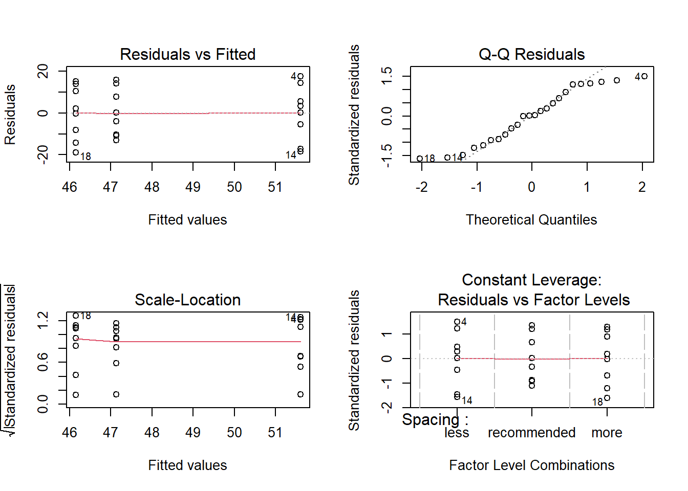
par(mfrow = c(1,1))2.1.2 A model with interactions
Working with the same dataset, let’s now look at a model with multiple predictors and their interaction. We will include block, Spacing and Nitrogen as fixed effects and the interaction between the last two:
fit2 <- lm(Yield ~ block + Spacing + Nitrogen + Spacing:Nitrogen, data = dat)
summary(fit2)
Call:
lm(formula = Yield ~ block + Spacing + Nitrogen + Spacing:Nitrogen,
    data = dat)

Residuals:
    Min      1Q  Median      3Q     Max
-6.8549 -1.2057  0.6726  2.6351  4.4577

Coefficients:
                             Estimate Std. Error t value Pr(>|t|)
(Intercept)                  51.22299    2.27402  22.525 4.25e-14 ***
block2                      -19.59212    1.48341 -13.208 2.29e-10 ***
Spacingrecommended            0.70175    3.04008   0.231   0.8202
Spacingmore                  -2.25521    3.04008  -0.742   0.4683
Nitrogen                      0.09051    0.01532   5.908 1.72e-05 ***
Spacingrecommended:Nitrogen  -0.04608    0.02167  -2.127   0.0484 *
Spacingmore:Nitrogen         -0.02853    0.02167  -1.317   0.2054
---
Signif. codes:  0 '***' 0.001 '**' 0.01 '*' 0.05 '.' 0.1 ' ' 1

Residual standard error: 3.634 on 17 degrees of freedom
Multiple R-squared:  0.935, Adjusted R-squared:  0.912
F-statistic: 40.73 on 6 and 17 DF,  p-value: 3.61e-09
Notice that Nitrogen is not a factor, so there is only a single coefficient for it (the slope of the relationship between Yield and Nitrogen for the reference levels of block and Spacing). In this case, the intercept of the model corresponds to the mean of the first (reference) levels of block and Spacing and value of Nitrogen equal to zero. Because the intercept has changed, the coefficients for Spacing and block are also now different from the previous model.
There are two coefficients for the interaction between Spacing and Nitrogen that correspond to the differences in the slope Yield vs Nitrogen between the second and third level of Spacing and the reference level of Spacing. Because we did not include an interaction term between block and Nitrogen, the effect of Nitrogen is assumed to be the same for both levels of block (and incidentally also for Spacing). That is, in this model we assume that the effect of block is additive and does not affect the relationship between Yield and the treatments.
Notice that the error of the model has decreased and the \(R^2\) has increased compared to the previous model. This is because the model is more complex and can explain more of the variation in the data. In general this will be true: the more complex the model, the better it will fit the data, unless the new predictors that are added are not related to the response variable. However, this does not mean that the model is better at predicting new data or that it is closer to reality, we might be capturing noise in the data (what is know as overfitting, we will discuss this later in the course).
Exercise 2.2
- What is the meaning of the F test at the end of the summary of the model we just fitted?
- Can you explain the degrees of the freedom of that F test?
Solution 2.2
The F test at the end of the summary tests the null hypothesis that all coefficients of the model (except the intercept) are zero. In other words, it tests whether the model is better than a model with only an intercept (i.e., the mean of the response variable).
The degrees of freedom of the F test are the degrees of freedom of the model and the residuals. The degrees of freedom of the model are the number of coefficients of the model (except the intercept) and the degrees of freedom of the residuals are the number of observations minus the number of coefficients of the model. In this case, the model has 6 coefficients (2 for
Spacing, 1 forblock, 1 forNitrogenand 2 for the interaction) and the residuals have 17 degrees of freedom (24 observations minus 6 coefficients and the intercept).
We can compute the marginal means for each level of Spacing as before. Notice that because Nitrogen is a continuous variable, rather than averaging over all possible values of Nitrogen we will instead calculate the marginal means for a specific value of Nitrogen (and average across the two blocks). For example, we can calculate the marginal means for Nitrogen = 0 since this is the reference value of Nitrogen:
emmeans(fit2, specs = c("Spacing"), at = list(Nitrogen = 0))NOTE: Results may be misleading due to involvement in interactions Spacing emmean SE df lower.CL upper.CL
less 41.4 2.15 17 36.9 46.0
recommended 42.1 2.15 17 37.6 46.7
more 39.2 2.15 17 34.6 43.7
Results are averaged over the levels of: block
Confidence level used: 0.95 Of course, this reference value is not necessarily meaningful in this context, so instead we could calculate the marginal means for a specific value of Nitrogen that is more meaningful. For example, we could calculate the marginal means for Nitrogen = 150:
emmeans(fit2, specs = c("Spacing"), at = list(Nitrogen = 150))NOTE: Results may be misleading due to involvement in interactions Spacing emmean SE df lower.CL upper.CL
less 55.0 1.41 17 52.0 58.0
recommended 48.8 1.41 17 45.8 51.8
more 48.5 1.41 17 45.5 51.4
Results are averaged over the levels of: block
Confidence level used: 0.95 Note that the warning message regarding interactions is generated automatically, it does not really mean that the analysis is wrong. In this case, we have set the value of Nitrogen (which is the variable with which Spacing interacts) so we have addressed the issue already.
Exercise 2.3
For the model with interaction, compute the marginal means for each level of
Spacingat the average level of Nitrogen, using emmeans. Try to confirm the marginal mean forSpacingmoreusing the coefficients of the model.Fit the same model again, but remove the interaction term. Calculate the marginal means at average nitrogen for this model. How do the results compare?
Now fit the marginal means for both models (with and without interaction) at 0 nitrogen. What do you notice?
Solution 2.3
- We can calculate the marginal means for each level of
Spacingas follows:
emmeans(fit2, specs = c("Spacing"), at=list(Nitrogen= 112.5))NOTE: Results may be misleading due to involvement in interactions Spacing emmean SE df lower.CL upper.CL
less 51.6 1.28 17 48.9 54.3
recommended 47.1 1.28 17 44.4 49.8
more 46.1 1.28 17 43.4 48.9
Results are averaged over the levels of: block
Confidence level used: 0.95 #By hand (for "more":
##(51.22299454+(51.22299454-19.59211565))/2-2.25521+ 0.09051274*112.5-0.02853*112.5- We can fit the model without the interaction term and calculate the marginal means as follows:
fit_noint <- lm(Yield~block+Spacing+Nitrogen, data = dat)
emmeans(fit_noint, specs = c("Spacing"), at=list(Nitrogen= 112.5))
Spacing emmean SE df lower.CL upper.CL
less 51.6 1.37 19 48.7 54.5
recommended 47.1 1.37 19 44.3 50.0
more 46.1 1.37 19 43.3 49.0
Results are averaged over the levels of: block
Confidence level used: 0.95 We can see that the marginal means are the same in both cases (although the the standard errors and confidence intervals differ), because we evaluate them at the same value of nitrogen which happens to be the average nitrogen in the data.
- If we now calculate the marginal means for both models at
Nitrogen = 0:
emmeans(fit2, specs = c("Spacing"), at=list(Nitrogen= 0))NOTE: Results may be misleading due to involvement in interactions Spacing emmean SE df lower.CL upper.CL
less 41.4 2.15 17 36.9 46.0
recommended 42.1 2.15 17 37.6 46.7
more 39.2 2.15 17 34.6 43.7
Results are averaged over the levels of: block
Confidence level used: 0.95 emmeans(fit_noint, specs = c("Spacing"), at=list(Nitrogen= 0)) Spacing emmean SE df lower.CL upper.CL
less 44.2 1.73 19 40.6 47.9
recommended 39.7 1.73 19 36.1 43.4
more 38.8 1.73 19 35.1 42.4
Results are averaged over the levels of: block
Confidence level used: 0.95 Now the marginal means are actually different (which are predictions outside of our data). This is because the interaction with Nitrogen causes different changes in yield at different spacings, as we move away from the mean level of Nitrogen.
2.2 Analysis of Variance
We can also perform an analysis of variance (ANOVA) on a fitted linear model using the anova function:
fit2 <- lm(Yield ~ block + Spacing + Nitrogen + Spacing:Nitrogen, data = dat)
anova(fit2)
Analysis of Variance Table
Response: Yield
Df Sum Sq Mean Sq F value Pr(>F)
block 1 2303.11 2303.11 174.4386 2.290e-10 ***
Spacing 2 135.79 67.90 5.1425 0.01793 *
Nitrogen 1 727.12 727.12 55.0725 9.993e-07 ***
Spacing:Nitrogen 2 60.86 30.43 2.3047 0.13012
Residuals 17 224.45 13.20
---
Signif. codes: 0 '***' 0.001 '**' 0.01 '*' 0.05 '.' 0.1 ' ' 1The ANOVA will distribute the total variance in the response variable across different terms including the residuals (as shown in the Sum Sq column). The rest of the table uses this sum of squares and the degreees of freedom to perform F tests for each term. Let’s calculate these terms by ourselves “manually” to illustrate how ANOVA works.
2.2.1 F test on the whole model
First, we compute the total sum of squares (SST) of the response variable:
y <- dat$Yield
SST = sum((y - mean(y))^2)
SST
[1] 3451.326Notice how SST only depends on the data, regardless of the model. The sum of squares of the model SSR is the same formula but applied to the values predicted (fitted) by the model for our sample. We can get these values from predict() or fitted():
y_hat <- fitted(fit2)
SSR2 <- sum((y_hat - mean(y_hat))^2)
SSR2
[1] 3226.875We can see that SSR2 < SST because the model is not able to explain all the variance in the data. The sum of squares of the residuals or error SSE2 is calculated analogously but now we assume that each prediction represents the estimated mean for each observation:
SSE2 <- sum((y - y_hat)^2)
SSE2
[1] 224.4504We can verify that SST = SSW + SSR:
SST == SSR2 + SSE2[1] TRUENotice how the value of SSE2 corresponds to the residual sum of squares in the ANOVA table. We can compute the mean squared error by dividing the sum of squares by the degrees of freedom of each term.
The degrees of freedom of the model are the number of coefficients of the model (except the intercept, so in this case 6) and the degrees of freedom of the residuals are the number of observations minus the number of coefficients of the model (in this case 17). The number of coefficients can be retrieved with length(coef(fit2)) or ncol(model.matrix(fit2)).
DF2 <- length(coef(fit2)) - 1
DFE2 <- length(y) - length(coef(fit2))
MSR2 <- SSR2 / DF2
MSE2 <- SSE2 / DFE2
c(MSR2, MSE2)
[1] 537.81254 13.20296Note that the mean squared errors are not additive:
MST2 <- SST / (length(y) - 1) # Equivalent to MSE of a model with only intercept
MST2 != MSR2 + MSE2
[1] TRUEAn F test for the entire model will compare the mean squared error of the model to the mean squared error of the residuals. The F statistic is the ratio of these two values:
F <- MSR2 / MSE2
F
[1] 40.73423This number correspond to the F statistic at the bottom of summary(fit2) (which we discussed before). The p-value of the F test can be calculated using the pf function that calculates the cumulative density of the F distribution. Notice how we need to pass the degrees of freedom of the two terms that were used to compute the F statistic:
1 - pf(F, df1 = DF2, df2 = DFE2)[1] 3.609712e-09And we can confirm that this is the same as the p-value for the F-statistic in summary(fit2).
2.2.2 F test to compare nested models
We can also perform an F test to compare two nested models. For example, we can compare the model with block, Spacing and Nitrogen to the model with just an intercept. This is equivalent to the F test we performed in the previous section (i.e., the F test of the whole model). Let’s first fit the model with just an intercept:
fit_null <- lm(Yield ~ 1, data = dat)As before, we can calculate the sum of squares of the residuals of the models:
y_hat_null <- fitted(fit_null)
SSE_null <- sum((y - y_hat_null)^2)
c(SSE2, SSE_null)
[1] 224.4504 3451.3256We can see that the sum of squared errors of the null model with only intercept is much larger than when we include predictors. This makes sense as the model with predictors is able to explain more of the variance in the data.
We can now calculate the F statistic to compare the two models. In this case, the denominator will be the mean squared error of the more complex model (MSE2, computed above). The numerator will be the related to the increase in squared error when going from the more complex to the simpler model:
DFE_null <- length(y) - length(coef(fit_null))
dSSE <- SSE_null - SSE2
dDF  <- DFE_null - DFE2
dMSE <- dSSE / dDF
dMSE
[1] 537.8125The F statistic is then:
F <- dMSE / MSE2
F
[1] 40.73423We can see that this is the same as the F statistic as the one at the end of the summary(fit2). Indeed, the F-statistic of the model is comparing a model with its nested versions where all predictors are dropped. We can generalize this to all possible nested models:
lm0<-lm(Yield~ 1,data=dat)
lm1<-lm(Yield~ block,data=dat)
lm2<-lm(Yield~ block+Spacing,data=dat)
lm3<-lm(Yield~ block+Spacing+Nitrogen,data=dat)
lm4<-lm(Yield~ block+Spacing+Nitrogen+Nitrogen:Spacing,data=dat)
If we extract the sum of squares of the residuals of each model:
SSE0 <- sum((dat$Yield - fitted(lm0))^2)
SSE1 <- sum((dat$Yield - fitted(lm1))^2)
SSE2 <- sum((dat$Yield - fitted(lm2))^2)
SSE3 <- sum((dat$Yield - fitted(lm3))^2)
SSE4 <- sum((dat$Yield - fitted(lm4))^2)
c(SSE0, SSE1, SSE2, SSE3, SSE4)
[1] 3451.3256 1148.2196 1012.4281 285.3085 224.4504If we now calculate the increments in sum of squared errors with respect to the more complex model:
dSSE <- c(SSE0 - SSE1, SSE1 - SSE2, SSE2 - SSE3, SSE3 - SSE4)
dSSE
[1] 2303.10597 135.79148 727.11961 60.85816These are the exact same values as in the Sum Sq column of the ANOVA table:
anova(fit2) # fit2 is the same as lm4Analysis of Variance Table
Response: Yield
Df Sum Sq Mean Sq F value Pr(>F)
block 1 2303.11 2303.11 174.4386 2.290e-10 ***
Spacing 2 135.79 67.90 5.1425 0.01793 *
Nitrogen 1 727.12 727.12 55.0725 9.993e-07 ***
Spacing:Nitrogen 2 60.86 30.43 2.3047 0.13012
Residuals 17 224.45 13.20
---
Signif. codes: 0 '***' 0.001 '**' 0.01 '*' 0.05 '.' 0.1 ' ' 1We can show the same for the degrees of freedom:
DFE0 <- length(dat$Yield) - length(coef(lm0))
DFE1 <- length(dat$Yield) - length(coef(lm1))
DFE2 <- length(dat$Yield) - length(coef(lm2))
DFE3 <- length(dat$Yield) - length(coef(lm3))
DFE4 <- length(dat$Yield) - length(coef(lm4))
c(DFE0 - DFE1, DFE1 - DFE2, DFE2 - DFE3, DFE3 - DFE4)
[1] 1 2 1 2Again, these are the same as the values in the column Df of the ANOVA table. We can see that all the ANOVA table is doing is comparing nested models that are built incrementally to the most complex model.
2.2.3 \(R^2\) and adjusted \(R^2\)
The \(R^2\) of the model is the proportion of the variance in the response variable that is explained by the model. It is calculated as the ratio of the sum of squares of the model to the total sum of squares:
R2 <- SSR2 / SST # Same as 1 - SSE2/SST
c(R2, summary(fit2)$'r.squared')
[1] 0.9349669 0.9349669The adjusted \(R^2\) is a modified version of the \(R^2\) that takes into account the degrees of freedom. It is calculated from the mean squared errors:
R2_adj <- 1 - MSE2/MST2 # Not MSR2/MST2!
c(R2_adj, summary(fit2)$'adj.r.squared')
[1] 0.9120141 0.9120141Note that the adjusted \(R^2\) is always smaller than the non-adjusted \(R^2\) and that the difference between the two increases with the number of predictors in the model.
Exercise 2.4
- Fit a model with
NitrogenandSpacing(including interaction) but withoutblock. - Perform an ANOVA and summary on the model.
- Compute the F-statistic of the model and for one of the predictors “manually” (like we did before for
fit2) and check your results with the output ofanova()andsummary(). - Compute the \(R^2\) and adjusted \(R^2\) of the model “manually” (like we did before for
fit2) and check your results with the output ofsummary().
Solution 2.4
- We fit the model without
block:
fit_nb <- lm(Yield ~ Spacing + Nitrogen + Spacing:Nitrogen, data = dat)- We perform an ANOVA and summary of the model:
anova(fit_nb)Analysis of Variance Table
Response: Yield
Df Sum Sq Mean Sq F value Pr(>F)
Spacing 2 135.79 67.90 0.4835 0.62439
Nitrogen 1 727.12 727.12 5.1782 0.03533 *
Spacing:Nitrogen 2 60.86 30.43 0.2167 0.80724
Residuals 18 2527.56 140.42
---
Signif. codes: 0 '***' 0.001 '**' 0.01 '*' 0.05 '.' 0.1 ' ' 1summary(fit_nb)
Call:
lm(formula = Yield ~ Spacing + Nitrogen + Spacing:Nitrogen, data = dat)

Residuals:
     Min       1Q   Median       3Q      Max
-16.6509  -8.9339  -0.0498   9.3362  14.0924

Coefficients:
                            Estimate Std. Error t value Pr(>|t|)
(Intercept)                 41.42694    7.01049   5.909 1.36e-05 ***
Spacingrecommended           0.70175    9.91433   0.071   0.9444
Spacingmore                 -2.25521    9.91433  -0.227   0.8226
Nitrogen                     0.09051    0.04996   1.812   0.0868 .
Spacingrecommended:Nitrogen -0.04608    0.07066  -0.652   0.5225
Spacingmore:Nitrogen        -0.02853    0.07066  -0.404   0.6911
---
Signif. codes:  0 '***' 0.001 '**' 0.01 '*' 0.05 '.' 0.1 ' ' 1

Residual standard error: 11.85 on 18 degrees of freedom
Multiple R-squared:  0.2677,    Adjusted R-squared:  0.06423
F-statistic: 1.316 on 5 and 18 DF, p-value: 0.3016- The F-statistic of the model can be done in two ways, either comparing the mean squared error of the model and residuals or by comparing the model to a nested one with only an intercept. Let’s do it in the first way:
y_hat_nb <- fitted(fit_nb)
# MSE of the model
SSR_nb <- sum((y_hat_nb - mean(y_hat_nb))^2)
DF_nb <- length(coef(fit_nb)) - 1
MSR_nb <- SSR_nb / DF_nb
# MSE of the residuals
SSE_nb <- sum((y - y_hat_nb)^2)
DFE_nb <- length(y) - length(coef(fit_nb))
MSE_nb <- SSE_nb / DFE_nb
# F-statistic
F_nb <- MSR_nb / MSE_nb
F_nb
[1] 1.315725We can now compute the p-value of the F-statistic:
1 - pf(F_nb, df1 = DF_nb, df2 = DFE_nb)[1] 0.3015519In the second way, we compare the model to a nested one with only an intercept:
# Fit null model and compute SSE and DF
fit_null <- lm(Yield ~ 1, data = dat)
y_hat_null <- fitted(fit_null)
SSE_null <- sum((y - y_hat_null)^2)
DF_null <- length(y) - length(coef(fit_null))
# Compute the F statistic for comparing nested models
dSSE <- SSE_null - SSE_nb
dDFE <- DF_null - DFE_nb
dMSE <- dSSE / dDFE
F_nb_null <- dMSE / MSE_nb
F_nb_null
[1] 1.315725- Compute the \(R^2\) and adjusted \(R^2\) of the model step-by-step and compare to the output by
summary().
# R2
SST_nb <- sum((y - mean(y))^2)
R2_nb <- SSR_nb / SST_nb
c(R2_nb, summary(fit_nb)$'r.squared')
[1] 0.2676564 0.2676564# Adjusted R2
MST_nb <- SST_nb / (length(y) - 1)
R2_adj_nb <- 1 - MSE_nb / MST_nb
c(R2_adj_nb, summary(fit_nb)$'adj.r.squared')[1] 0.06422757 0.064227572.3 Simulating the sampling distribution
In previous sections we have calculated the standard errors of different estimates but what exactly do these numbers mean? Of course, the standard error is a measure of the uncertainty of the estimate but more specifically, it is estimating the standard deviation of the sampling distribution of the estimate (see appendix on statistical inference for details). In this section we will approximate the sampling distribution of the estimates of a linear model by simulating from the fitted model.
We will use the model with block, Spacing and Nitrogen as predictors and we will simulate the sampling distribution for the coefficient of Spacingmore. We can simulate new data from a fitted model using the function simulate():
fit2 <- lm(Yield ~ block + Spacing + Nitrogen + Spacing:Nitrogen, data = dat)
nsim = 5000
sim <- simulate(fit2, nsim = nsim)
The argument nsim specifies the number of simulations that we want to perform. The output of simulate() is a matrix where each column represents a different simulation of the response variable:
cbind(sim[,1:5], dat$Yield) sim_1 sim_2 sim_3 sim_4 sim_5 dat$Yield
1 55.03805 54.36874 51.32974 51.80462 53.06795 51.84274
2 57.62836 57.63781 59.08455 58.75735 59.77640 57.20000
3 59.70434 63.10647 70.00761 68.14054 61.84072 66.00000
4 70.41176 73.79261 72.89583 76.77949 70.38536 69.20000
5 48.31838 53.23775 51.10207 45.61208 51.24152 48.21026
6 50.85416 54.48578 48.23536 62.06495 53.11198 56.72479
7 53.72647 56.75551 51.92627 59.09356 58.02993 61.17094
8 64.21166 58.62573 68.54755 63.59279 60.31920 60.09573
9 50.18924 56.91899 50.89458 52.99670 54.47867 47.36752
10 54.52945 55.80121 60.13806 52.49281 59.56028 54.98120
11 56.75070 55.98243 59.54268 53.49076 58.04150 62.88547
12 59.68436 63.58012 56.55523 66.12293 61.67455 61.40000
13 24.70377 30.01173 31.31653 36.00661 32.63080 34.33423
14 39.67961 38.43229 39.78165 42.23851 41.65075 33.20000
15 46.17445 50.55390 49.51535 44.97151 44.17604 46.10000
16 52.38784 54.53489 48.13632 50.87762 52.56589 55.00000
17 24.51909 25.83707 27.46984 32.81325 18.20408 31.90349
18 37.41796 38.92119 33.23154 39.68220 31.27665 27.16956
19 36.13633 41.41601 37.07460 31.77956 48.54382 37.95012
20 47.38848 46.50393 39.67482 42.35287 43.84978 45.93434
21 26.39860 32.36843 34.19636 31.09437 32.99461 36.79029
22 34.91859 33.10478 35.58651 38.58625 36.68002 36.39021
23 34.98301 33.06094 43.65753 42.29497 44.15233 34.10000
24 39.08118 43.42457 39.45248 41.32387 35.19913 43.10101Each column of sim is a different possible outcome of the same experiment with the same treatments and conditions. Of course, we are using the estimate of the coefficients of the model (rather than the true coefficients) so this is only an approximation. We can reconstruct the sampling distribution of any coefficient by fitting the model to each of the simulated datasets and extracting the coefficient of interest. Let’s do that for Spacingmore:
sample_distribution <- numeric(nsim) # Create an empty vector to store the estimates
# Loop over all the simulations
for (i in 1:nsim) {
    # Fit model using simulated yield rather than original one
    y_sim <- sim[,i]
    fit_sim <- lm(y_sim ~ block + Spacing + Nitrogen + Spacing:Nitrogen, data = dat)
    # Extract the coefficient of interest
    sample_distribution[i] <- coef(fit_sim)["Spacingmore"]
}
We can plot the sampling distribution of the coefficient of Spacingmore with the original estimate on top of it:
hist(sample_distribution, breaks = 25, freq = FALSE)
abline(v = coef(fit2)["Spacingmore"], col = "red")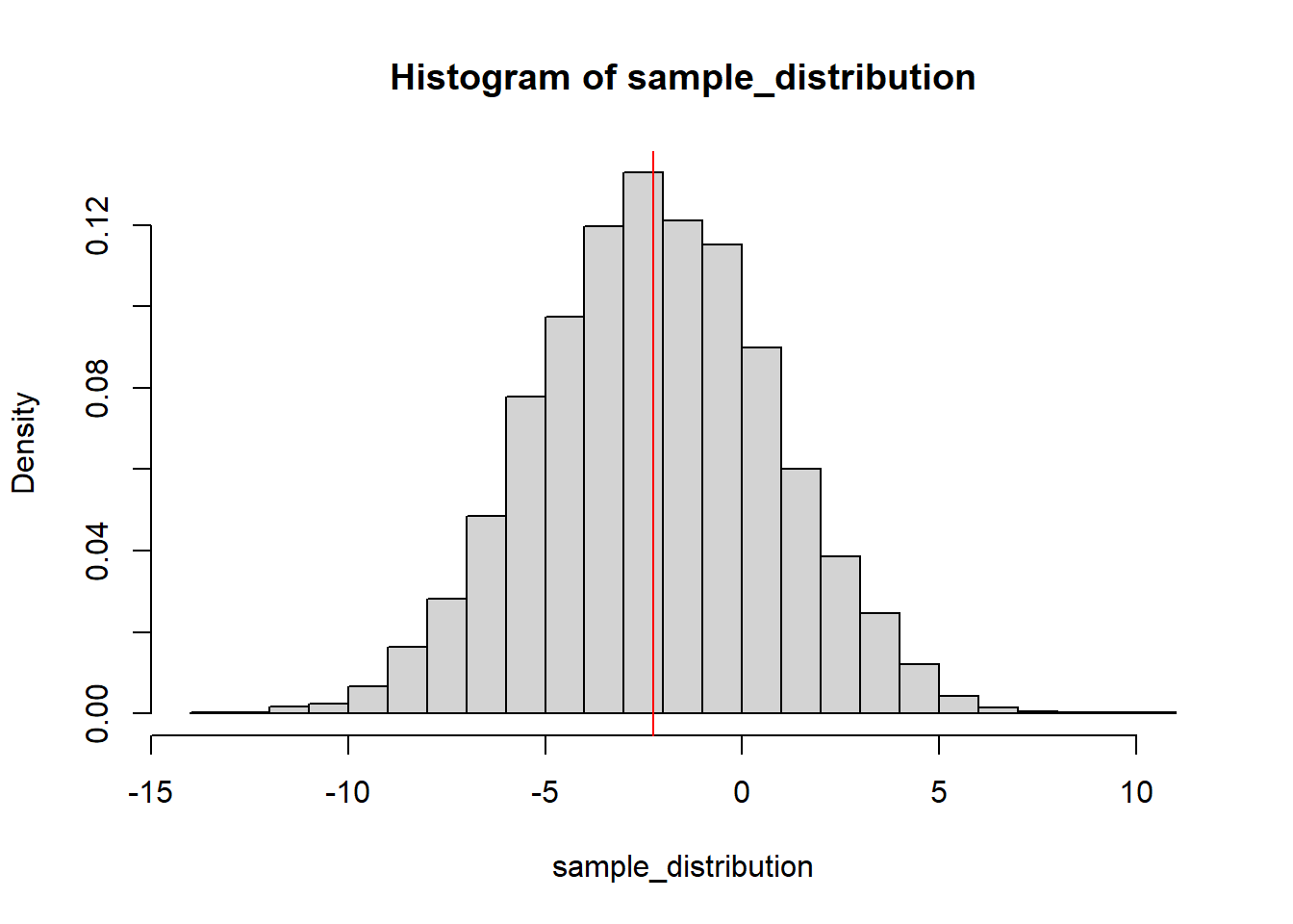
The theory says that the t-statistic of the estimate of the coefficient of Spacingmore should follow a t distribution with 17 degrees of freedom (the residual degrees of freedom of the model). We can compare the histogram of the sampling distribution to the t-distribution:
sample_t = (sample_distribution - mean(sample_distribution))/sd(sample_distribution)
hist(sample_t, breaks = 25, freq = FALSE)
curve(dt(x, df = 17), col = "red", add = TRUE)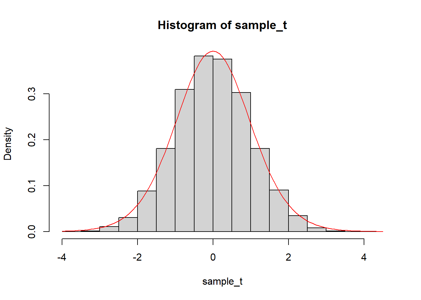
We can see that the simulated distribution does match the theory. The standard deviation of the simulated distribution is then also very similar to the standard error of the estimate:
sd(sample_distribution)[1] 3.010348summary(fit2)$coefficients["Spacingmore", "Std. Error"][1] 3.040078The small difference is due to the fact that we are calculating the standard deviation of the simulated sampling distribution from a finite number of simulations. The larger the number of simulations, the closer the standard deviation of the simulated distribution will be to the standard error of the estimate.
Exercise 2.5
Simulate the sampling distribution of the coefficient of
Spacingrecommended:Nitrogen and compare it to the theoretical t-distribution and the standard error of the estimate.
Solution 2.5
We can reuse the simulated dataset from before, we just need to change the coefficient of interest in the model:
sample_distribution <- numeric(nsim) # Create an empty vector to store the estimates
# Loop over all the simulations
for (i in 1:nsim) {
    # Fit model using simulated yield rather than original one
    y_sim <- sim[,i]
    fit_sim <- lm(y_sim ~ block + Spacing + Nitrogen + Spacing:Nitrogen, data = dat)
    # Extract the coefficient of interest
    sample_distribution[i] <- coef(fit_sim)["Spacingrecommended:Nitrogen"]
}
We can compare the histogram of the sampling distribution to the t-distribution:
sample_t = (sample_distribution - mean(sample_distribution))/sd(sample_distribution)
hist(sample_t, breaks = 25, freq = FALSE)
curve(dt(x, df = 17), col = "red", add = TRUE)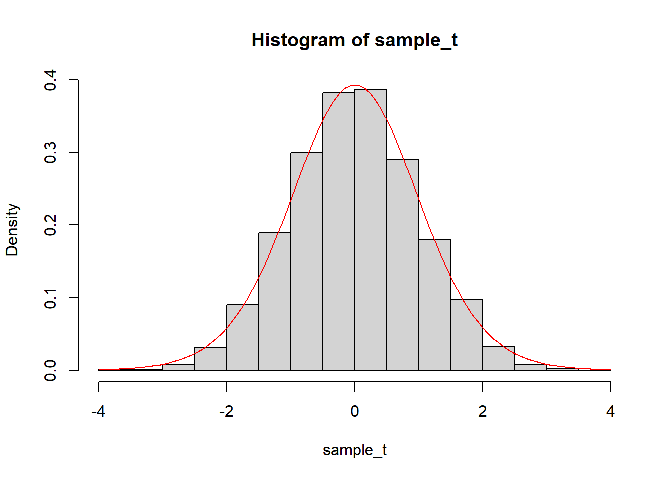
We can also compare the standard deviation of the simulated distribution to the standard error of the estimate:
sd(sample_distribution)[1] 0.02191149summary(fit2)$coefficients["Spacingrecommended:Nitrogen", "Std. Error"][1] 0.02166653