Let’s simulate some data of a similar nature to the one obtained from the case study on banana in Uganda. We will assume a number of locations (n) and observations per location (r). A covariate x is generated with one value per farm.
Let’s build the model. The design matrices for the fixed and random effects are as follows:
X <-matrix(sim.data$x, ncol =1)Z <-model.matrix(~location-1, data = sim.data)
The vectors of coefficients and random effects are:
# Fixed effectsmu <-0# Overall mean in logit scaleBeta <-0.15# Slope with respect to X in logit scale# Random effectssigma.b <-1# Standard deviation of random effects on mean in logit scaleb <-rnorm(n,mean =0,sd = sigma.b) # Random effects on mean in logit scale
Now we generate the response variable y:
library(boot) # for inverse logit# Mean in logit scalesim.data$y.mu <- mu+X%*%Beta+Z%*%b# Proportion in original scalesim.data$p <-inv.logit(sim.data$y.mu)# Simulate individual observations by sampling from Binomial distribution with n = 1 and psim.data$y <-rbinom(n*r, size =1, prob = sim.data$p)
Now we can fit a generalized linear model to this data. As shown in the lectures, we will use the function glmer from the lme4 package and specify a binomial distribution:
library(lme4)
Loading required package: Matrix
library(lmerTest)
Attaching package: 'lmerTest'
The following object is masked from 'package:lme4':

    lmer
The following object is masked from 'package:stats':

    step
glmm1 <-glmer(y ~ x + (1|location), data = sim.data, family ="binomial")
Exercise 9.1
Check the estimates of the fixed effects and the random effects in the model and discuss the results considering the values of the parameters used to simulate the data.
Calculate the predictions of intercept for each location (tip: use predict() or the functions ranef() and fixef()) in the original scale.
Add the effect of x to the predictions and plot the predictions against the true
Solution 9.1
We can retrieve the estimates using summary():
summary(glmm1)
Generalized linear mixed model fit by maximum likelihood (Laplace
  Approximation) [glmerMod]
 Family: binomial  ( logit )
Formula: y ~ x + (1 | location)
   Data: sim.data

      AIC       BIC    logLik -2*log(L)  df.resid
    254.0     263.9    -124.0     248.0       197

Scaled residuals:
    Min      1Q  Median      3Q     Max
-2.1599 -0.8229  0.3687  0.7546  1.8467

Random effects:
 Groups   Name        Variance Std.Dev.
 location (Intercept) 0.6393   0.7996
Number of obs: 200, groups:  location, 20

Fixed effects:
            Estimate Std. Error z value Pr(>|z|)
(Intercept)  0.09139    0.24305   0.376  0.70691
x            0.12527    0.04058   3.087  0.00202 **
---
Signif. codes:  0 '***' 0.001 '**' 0.01 '*' 0.05 '.' 0.1 ' ' 1

Correlation of Fixed Effects:
  (Intr)
x -0.118
The true value for the intercept was mu = 0, so the estimate is quite good. The slope with respect to x was Beta = 0.15, and the estimate is 0.18 so the slope was also well estimated. The standard deviation of the random effects was sigma.b = 1, and the estimate is 0.78, which is not too far from the true value although somewhat underestimated.
We can calculate the predictions of the mean for each location using predict() by setting x = 0 and location as a factor with levels 1 to n:
pred <-predict(glmm1, newdata =data.frame(x =0, location =factor(1:n)))pred.p <-inv.logit(pred)
We could also use ranef() and fixef() to calculate the predictions:
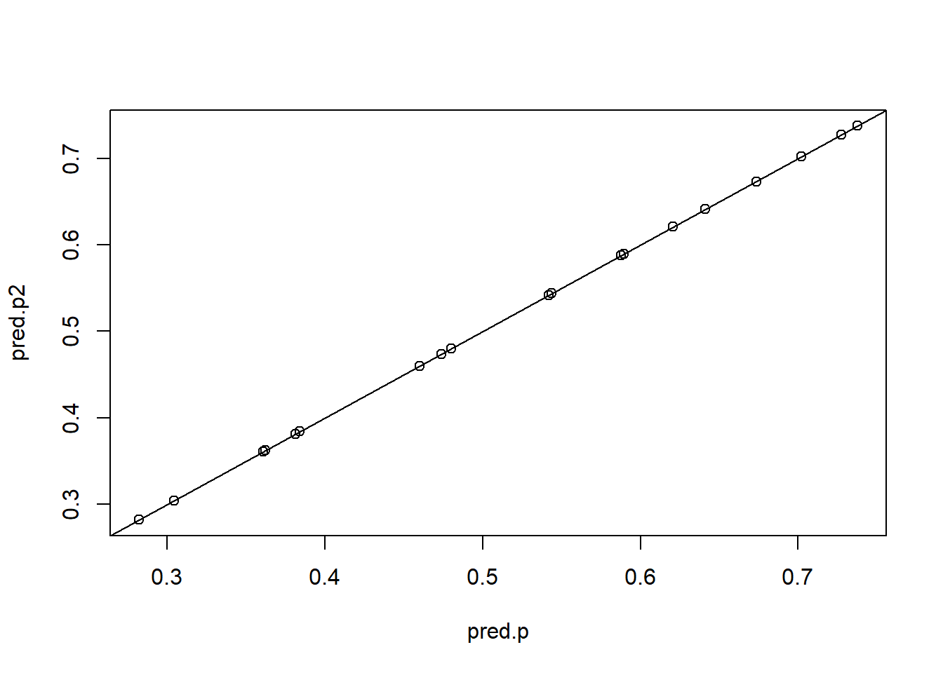
ranef.glmm1 <-ranef(glmm1)fixef.glmm1 <-fixef(glmm1)pred.p2 <-inv.logit(fixef.glmm1[1] + ranef.glmm1$location[,1])plot(pred.p, pred.p2)abline(a =0, b =1)
We could just use predict() to include predictions for every observation in the original scale:
sim.data$p.pred <-predict(glmm1, type ="response")
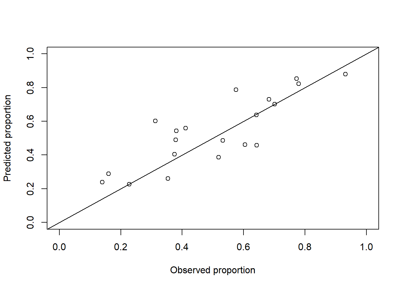
plot(p.pred~p, xlab ="Observed proportion", ylab ="Predicted proportion",xlim =c(0,1), ylim =c(0,1), data = sim.data)abline(a =0, b =1)
We can also reconstruct the predictions from the fixed and random effects:
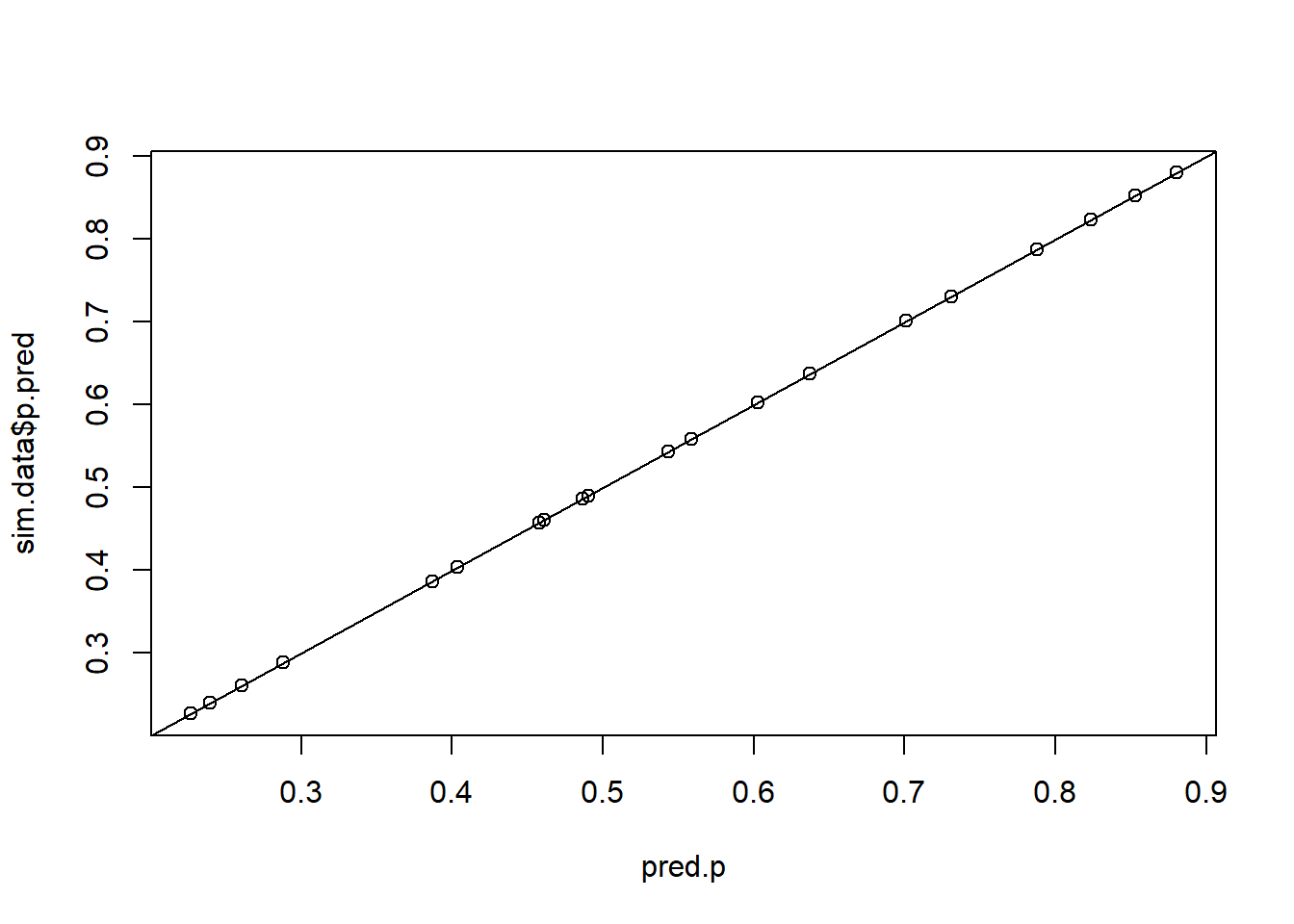
x_sorted <-unique(sim.data$x)pred.p <-rep(inv.logit(fixef.glmm1[1] + ranef.glmm1$location[,1] + x_sorted*fixef.glmm1[2]), each = r)plot(pred.p, sim.data$p.pred)abline(a =0, b =1)
9.2 Using Poisson distribution
Let’s now simulate data using a Poisson distribution and a log link function but following the same steps as before. In this case n = 30 and r = 5:
The design matrices for the fixed and random effects are the same:
X <-matrix(sim.data$x, ncol =1)Z <-model.matrix(~location-1, data = sim.data)
The vectors of coefficients and random effects are:
# Fixed effectsmu <-0# Overall mean in log scaleBeta <-0.15# Slope with respect to X in log scale# Random effectssigma.b <-1# Standard deviation of random effects on mean in log scaleb <-rnorm(n,mean =0,sd = sigma.b) # Random effects on mean in log scale
Now we generate the response variable y using rpois():
# Mean in log scalesim.data$y.mu <- mu+X%*%Beta+Z%*%b# Proportion in original scalesim.data$lambda <-exp(sim.data$y.mu)# Simulate individual observations by sampling from Binomial distribution with n = 1 and psim.data$y <-rpois(n*r, lambda = sim.data$lambda)
Now we can fit a generalized linear model to this data and specify a Poisson distribution:
glmm1 <-glmer(y ~ x + (1|location), data = sim.data, family ="poisson")
Exercise 9.2
Check the estimates of the fixed effects and the random effects in the model and discuss the results considering the values of the parameters used to simulate the data.
Calculate the predictions of intercept for each location (tip: use predict() or the functions ranef() and fixef()) in the original scale.
Add the effect of x to the predictions and plot the predictions against the true
Solution 9.2
We can retrieve the estimates using summary():
summary(glmm1)
Generalized linear mixed model fit by maximum likelihood (Laplace
  Approximation) [glmerMod]
 Family: poisson  ( log )
Formula: y ~ x + (1 | location)
   Data: sim.data

      AIC       BIC    logLik -2*log(L)  df.resid
    494.5     503.5    -244.3     488.5       147

Scaled residuals:
    Min      1Q  Median      3Q     Max
-1.6669 -0.6848 -0.1970  0.5163  2.2707

Random effects:
 Groups   Name        Variance Std.Dev.
 location (Intercept) 0.7104   0.8428
Number of obs: 150, groups:  location, 30

Fixed effects:
            Estimate Std. Error z value Pr(>|z|)
(Intercept)  0.14720    0.18447   0.798  0.42490
x            0.09060    0.03013   3.007  0.00263 **
---
Signif. codes:  0 '***' 0.001 '**' 0.01 '*' 0.05 '.' 0.1 ' ' 1

Correlation of Fixed Effects:
  (Intr)
x -0.310
The true value for the intercept was mu = 0, so the estimate is quite good. The slope with respect to x was Beta = 0.15, and the estimate is 0.09 so the slope was somewhat well well estimated. The standard deviation of the random effects was sigma.b = 1, and the estimate is 0.71, which is not too far from the true value although somewhat underestimated.
We can calculate the predictions of the mean for each location using predict() by setting x = 0 and location as a factor with levels 1 to n:
pred <-predict(glmm1, newdata =data.frame(x =0, location =factor(1:n)))pred.lambda <-exp(pred)
We could also use ranef() and fixef() to calculate the predictions:
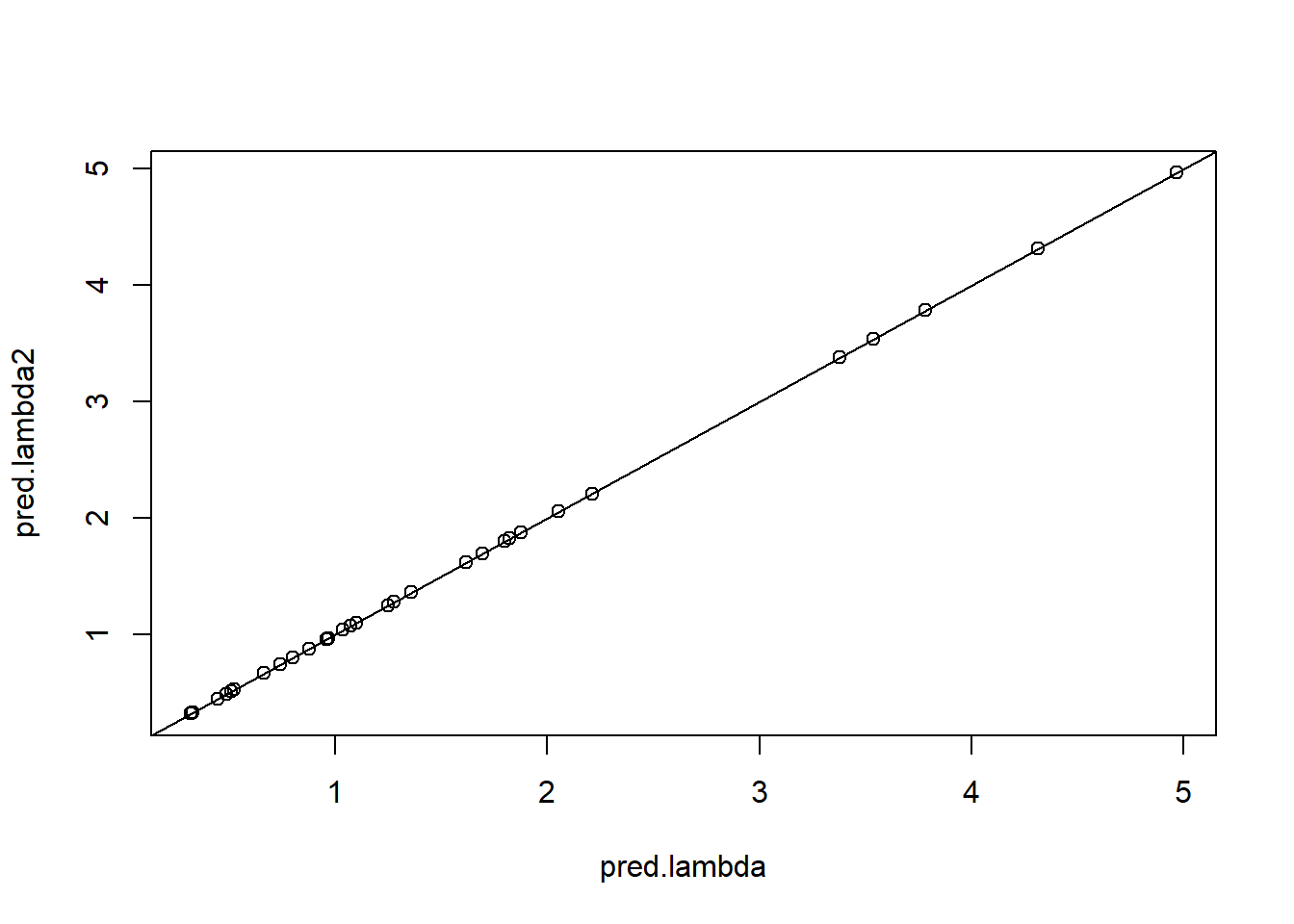
ranef.glmm1 <-ranef(glmm1)fixef.glmm1 <-fixef(glmm1)pred.lambda2 <-exp(fixef.glmm1[1] + ranef.glmm1$location[,1])plot(pred.lambda, pred.lambda2)abline(a =0, b =1)
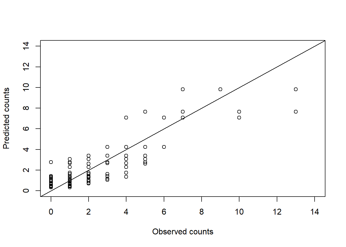
We could just use predict() to include predictions for every observation in the original scale:
sim.data$y.pred <-predict(glmm1, type ="response")
plot(y.pred~y, xlab ="Observed counts", ylab ="Predicted counts",xlim =c(0,14), ylim =c(0,14), data = sim.data)abline(a =0, b =1)
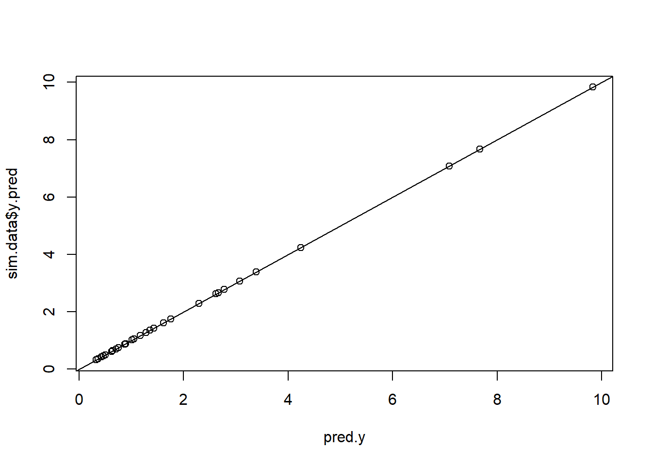
We can also reconstruct the predictions from the fixed and random effects:
x_sorted <-unique(sim.data$x)pred.y <-rep(exp(fixef.glmm1[1] + ranef.glmm1$location[,1] + x_sorted*fixef.glmm1[2]), each = r)plot(pred.y, sim.data$y.pred)abline(a =0, b =1)